Numerical accuracy and convergence#
Where solprop stands on accuracy, in one place: every convergence study and every
comparison against Luna or an analytic answer, with the number, the case it was measured
on and the test that holds it. Every ladder here writes its rungs to a small JSON
record under tests/data/convergence/, committed like a witness and compared against
on every later run, and the figures are drawn from those files (section 9). The tables
carry the scalar results; the figures carry the ladders. A number here without a test
behind it is a defect of the page.
Conventions throughout. “Shape” is the relative L2 distance between two in-band spectral
energy densities; “content” is the ratio of their in-band integrals. Luna is the
modal-fixed checkout at de9db7c9 unless stated, driven read-only by the generators
under tests/data/. The named cases (M1, M2/RDW, M4/CtC) are defined in
testing.md §8.
Luna comparisons and true power. solprop’s modal amplitudes are true-power
amplitudes and its run statistics analytic Poynting flux (ADR-030); Luna’s are
vacuum-normalised. Luna’s stored spectra are therefore converted by the solprop mode’s
sqrt(Re n_eff(ω, z_plane)) at their saved positions before comparison, with the
conversion built from Luna’s own archived cladding and gas data, and the witness runs
launch the true energy of Luna’s pulse — the nominal energy times the
launch-spectrum-weighted mean of Re n_eff(ω, 0), 1.0000357 for the reduced M2 case
and 1.0049222 for the reduced CtC case. That mean agrees with the true energy of the
archives’ own plane zero to 2e-16 on both RDW cases and the full CtC one, and to 1.2e-11
on the reduced CtC one. The three curves read from luna_rdw_switches.json carry scalar
energies without spectra, so they keep the vacuum-norm diagnostic on both codes and are
not physical Poynting energies.
1. The integrators and the tables#
what |
measured |
where |
|---|---|---|
DOPRI5 order on a scalar ODE |
observed order 4.5–5.5 on the solution, 3.5–4.5 on the embedded pair, over a fixed-step ladder to 64 steps, at the round-off floor beyond |
|
Chebyshev builds |
exact on polynomials; error bound met on the ladder of tolerances; array-valued build equals per-column scalar builds |
|
cumulative operator Φ against |
4.8e-12 for the expansion and 2.5e-12 for the z table on the RDW gradient capillary; on the acceptance test’s own 0.2 m gradient fixture (optmat’s helium), 4.6e-11 and 1.4e-10 over twenty random intervals, each asserted below its interval’s bound: the tolerance the table is built to, |
|
the round-off floor of one evaluation of |
~1e-11 relative, the frame’s own cancellation of eight digits; measured per element in the acceptance test’s norm (2.27e-7 on the M2 capillary with its absorber) and applied as |
|
the parameter expansion against the z table |
9.8e-10 on the RDW capillary, 4.9e-9 on the reduced M2 case, 5.0e-9 at the CtC size, every one two orders inside the tolerance both are built to |
|
ionisation rate tables |
relative error falls at fourth order as the knots double; 1e-6 relative at 257 knots for optmat’s PPT form of every noble gas |
|
the plasma column’s cumulative trapezoid |
second order in the sample spacing on a constant field: 9.9e-5 at 8193 samples, falling by four at each doubling; a pre-ionised tone has the Drude susceptibility times the two integrals’ multiplier, \(((\theta/2)\cot(\theta/2))^2\), to round-off — 3.7e-8 short of it at \(\theta = 4.7\times10^{-4}\), 0.8225 of it at the default grid’s \(\omega_{\max}\) and 0.7866 at \(1.1\,\omega_{\max}\) (below) |
|
the plasma column’s band rule (SEP 18) |
the composite multiplier within a certified \(10^{-5}\) of one across the active band; on ionising fields \(\le 6.5\times10^{-6}\) per band against an independent reference, and over ten propagation steps \(\le 4.2\times10^{-6}\) (below) |
|
the Raman kernel’s normalisation |
analytic against quadrature; the dephasing-capped decay exponent; the window residual reported at debug level |
|
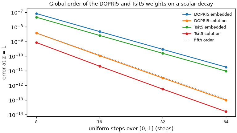
The global order of both tableaux on y' = -y, four levels each for the solution and the embedded weights, from tests/data/convergence/tableau_order.json (written by tests/stepper/test_tableau.py). Every rung is above the round-off floor the ladder guards against, and the fifth-order reference is drawn through DOPRI5’s coarsest.#
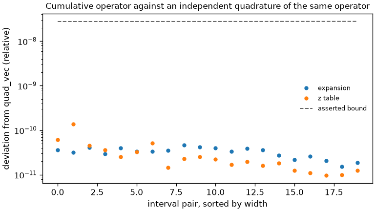
The cumulative operator against quad_vec on the same twenty random intervals, for both representations, from tests/data/convergence/phi_quadrature.json (tests/translate/test_linop.py). The dashed line is each interval’s bound, which both are asserted against.#
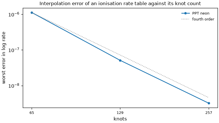
The ionisation rate table’s worst error against its knot count, on optmat’s PPT form of neon’s rate (ppt_ilkov), from tests/data/convergence/ionisation_knots.json (tests/translate/test_ionisation_tables.py). The dotted line is fourth order, the interpolation order of the cubic.#
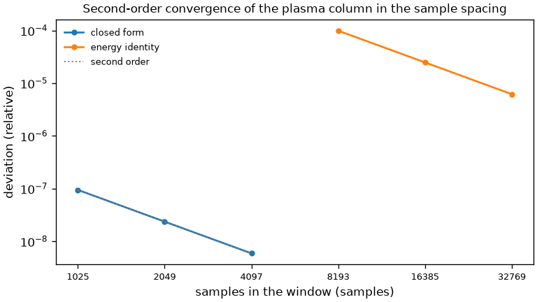
The plasma column’s two second-order ladders – the closed-form polarisation and the energy identity – from tests/data/convergence/plasma_trapezoid.json (tests/nonlinear/test_plasma.py). The dotted line is second order, the trapezoid’s.#
The plasma column at the top of the band. The second-order ladder above is measured on
a constant field. On an oscillating integrand the trapezoid’s error is a
frequency-dependent multiplier instead. For a sampled tone \(e^{i\omega t}\) the cumulative
trapezoid returns \(-i(\delta t/2)\cot(\omega\,\delta t/2)\,e^{i\omega t}\) plus an
integration constant, where the exact antiderivative has \(-i/\omega\). The ratio
\((\theta/2)\cot(\theta/2)\), with \(\theta = \omega\,\delta t_{\rm fine}\), is real: it scales
the amplitude and leaves the phase alone. It is \(1 - \theta^2/12 + O(\theta^4)\), second
order as the ladder says, but the field grid’s rule
\(\delta t_{\rm fine} = 2\pi/(f_{\rm fac}\,\omega_{\max})\) puts the top of the band at
\(\theta = 2\pi(\omega/\omega_{\max})/f_{\rm fac}\), which is \(\pi/3\) at \(\omega_{\max}\) with
the default ffac = 6. A physical-polarisation evaluation applies the rule three times: the exposure gives \(f\),
\(\int fE\) gives \(J_{\rm free}\), and \(\int(J_{\rm free} + J_{\rm loss})\) gives \(P\). The loss
current goes through one integral and the Drude term through two. The production
column stops at the current and forms the held source in frequency
(SEP 27): its interior Drude multiplier
has one integration factor, and its loss current has none. The two-integral values
below qualify the direct physical response:
\(\omega/\omega_{\max}\) |
\(\theta\) at |
one integral |
two (Drude) |
one, |
two, |
|---|---|---|---|---|---|
0.5 |
0.524 |
0.977 |
0.955 |
0.948 |
0.899 |
0.75 |
0.785 |
0.948 |
0.899 |
0.882 |
0.777 |
1.0 |
1.047 |
0.907 |
0.822 |
0.785 |
0.617 |
1.1 (collar top) |
1.152 |
0.887 |
0.787 |
0.738 |
0.544 |
The two-integral identity on a pre-ionised tone is exact to round-off and held by
tests/nonlinear/test_plasma.py. That is the trapezoid rule, integration="trapezoid",
which the comparisons with Luna use. The band rule of
SEP 18 filters each integrand with taps
designed for the grid (field plasma).
It brings the composite multiplier to within a certified \(10^{-5}\) of one across the
active band: \(K = 4\) and \(4.92\times10^{-6}\) at ffac = 6, \(K = 7\) at ffac = 4. It is
refused below ffac ≈ 3.55. Its records, all on numpy_ref, follow.
The ten-step propagation record uses the held-current source and records that
equation explicitly; the response records are of the physical polarisation.
study |
band rule ( |
trapezoid ( |
where |
|---|---|---|---|
interior Drude susceptibility of a pre-ionised tone at 0.5, 1.0 and 1.0999 \(\omega_{\max}\) |
within \(2\varepsilon + \varepsilon^2\) (\(9.8\times10^{-6}\) at the top) |
0.955, 0.822, 0.787 of it |
|
whole-window error of a band-limited tone starting at \(\lambda\) of its peak, 4096 samples |
\(3.8\times10^{-6}\) at \(\lambda = 10^{-8}\); \(\kappa = 30\)–33 for \(\lambda = 10^{-6}\)–\(10^{-4}\) |
0.18 |
|
closed-form constant-field ladder |
\(8.7\times10^{-11}\) at 1025 samples, falling by 5.4 and 4.8 |
\(9.5\times10^{-8}\), falling by 4 |
|
energy identity ladder |
\(4.4\times10^{-8}\) at 8193 samples, second order |
\(9.9\times10^{-5}\), second order |
|
polarisation of five ionising fields (He and Ar, weak to saturating, a 30 fs pulse) against Richardson (48, 96) |
asserted bands \(\le 6.5\times10^{-6}\), active band \(\le 1.8\times10^{-6}\) |
\(1.2\times10^{-2}\) to \(1.6\times10^{-1}\) per band, \(4.7\times10^{-4}\) to \(6.0\times10^{-3}\) active |
|
held-current plasma-induced change over ten capillary steps against Richardson (48, 96) |
\(\le 3.9\times10^{-6}\) (He) and \(\le 1.2\times10^{-6}\) (Ar) per band; active \(6.0\times10^{-7}\) and \(5.1\times10^{-7}\) |
0.98–6.9 % per band; active \(2.8\times10^{-3}\) and \(2.9\times10^{-3}\) |
|
The two qualification studies. Their protocols are complete in SEP 18 §7, items 4 and 5, and in the tests that write the records.
The reference. It is the trapezoid column itself, refined and extrapolated: \(R = (4P_{96} - P_{48})/3\). With
pow2sizes the coarse axis is unchanged under refinement, so spectra compare bin for bin. The reference uses no band filter or spectral floor. The ten-step comparison uses the same held-current assembly on each grid and isolates the current integral’s accuracy; SEP 27’s analytic tests independently qualify that assembly.Its uncertainty. The same extrapolation from 24 and 48 agrees with it to \(\le 8.2\times10^{-6}\) per band and \(\le 6.4\times10^{-9}\) over the active band at the response level. Over the ten held-current steps the largest asserted-band reference uncertainties are \(3.6\times10^{-7}\) (He) and \(7.1\times10^{-7}\) (Ar), and the active-band uncertainties are \(1.2\times10^{-8}\) and \(8.9\times10^{-9}\).
Which bands are asserted. A band is asserted where it holds at least \(10^{-6}\) of the active band’s share and recorded otherwise.
The one recorded band above \(10^{-4}\). The 30 fs argon pulse’s collar, at \(2\times10^{-4}\), holds \(1.7\times10^{-8}\) of the response. It falls a thousandfold at
ffac = 12under the same rule, so it is the sampling of the products \(fE\) and \(W\), not the integration.With the plasma off, every
ffacagrees to \(10^{-12}\), which is asserted.The diagnostics. The work defect is \(\le 4.7\times10^{-8}\) under the band rule, against up to \(5.3\times10^{-4}\) for the trapezoid. The undershoot is \(\le 2.2\times10^{-4}\).
What it means: under the trapezoid, plasma dispersion and ionisation loss acting on content near \(\omega_{\max}\) are 10–20 % too weak. That includes a vacuum-ultraviolet dispersive wave on a grid whose short limit sits just below it. A pump at a quarter of \(\omega_{\max}\) or below sees at most about 1 %. The band rule removes the error to the records above, for the cost of a nine-tap filter per integrand on the default grid, and is the default (SEP 18 §11).
The envelope route’s plasma and the TDSE current stream convert their currents with exact inverse-frequency factors and do not have this multiplier (algorithms.md, ionisation). The accepted SEP 17 §4.3 proposes a continuum polarisation directly, avoiding an extra current integral; its §4.6 requires a discrete source-work qualification, and its pump-plasma baseline uses the existing band rule. The proposed continuum response is not yet implemented or qualified.
2. The transverse quadrature#
The transverse integral of the nonlinear polarisation is a fixed rule (ADR-010); its accuracy is measured, not adapted, and the alarm is a statistic.
study |
result |
where |
|---|---|---|
alarm against radial order, three HE₁ₘ modes |
2.365e-1, 3.316e-2, 1.451e-4, 1.777e-8, 4.224e-15 at n_r = 8, 16, 24, 32, 48; the 1e-6 threshold separates 24 from 32 |
|
what an alarm of 1.0e-1 costs |
the M2 VUV band wrong by 6.6e-5 ( |
|
the Kerr overlap tensor |
solprop’s projected drive is the analytic quartic overlap of the Bessel profiles to 8.9e-16 (two modes) and 1.6e-13 (four): 0.4785422894, 0.0221346036, −0.0023723438 for modes 2–4 |
|
Luna’s own projection of the same field |
the same overlaps to 1.9e-12 at 64, 128 and 256 nodes, with and without Kronrod; its discrete Gram matrix the identity to 8.9e-16 |
|
the M2 quadrature ladder |
n_r = 32, 64, 128 leave the second mode’s exit energy unchanged to seven digits on both codes |
|
the alarm on the milestone runs |
≤ 1.0e-6 over the M2 planes where it is defined, |
|
the default radial order |
|
|
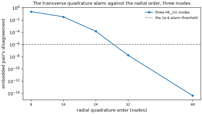
The alarm against the radial order on a three-mode set, from tests/data/convergence/quadrature_alarm.json (tests/backends/test_numpy_ref_multimode.py). The dashed line is the 1e-6 threshold at which the backend warns; it falls between 24 and 32 nodes, which is why a mode set takes the higher default that a single HE11 does not.#
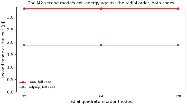
The second mode’s exit energy of the full M2 case against the radial order, on both codes, from tests/data/convergence/m2_quadrature.json (tests/driver/test_prop_capillary.py). Neither code moves to seven digits, which is what excludes the transverse rule as a cause of the difference between them; Luna’s rows are read from tests/data/luna_rdw_switches.json and no Luna is run.#
3. Agreement with Luna at the level of a kernel#
Each row is a witness generated by Luna itself and stored under tests/data/, or a direct
transcription check. These are the numbers that say the physics is the same before a
propagation compares the two codes.
quantity |
agreement |
where |
|---|---|---|
the plasma response (current and loss term) |
5.4e-14 after the CODATA rescaling |
|
Raman lines (rotational, vibrational) |
5e-6 (the ħ/k_B CODATA shift) and round-off; the whole hydrogen response 3.8e-5 once Luna’s own 70 % taper is applied to solprop’s kernel |
|
the linear operator on a constant capillary, both grids |
residual below 1e-10 against |
|
the mode-averaged prefactor |
1e-13 once the CODATA 2014/2022 difference in ε₀ is accounted for |
|
Vincetti constant-tube index and loss, Luna’s form of the fits ( |
3.06e-16 absolute in |
|
Vincetti production form against converged JCMwave FEM rows (30 µm core, 180 nm walls, six tubes; t/r = 0.017, outside the fits’ range) |
index RMSE 7.5e-6 over 79 vacuum rows, 2.9 % of the decrement median away from resonance; 4.5e-6 and 0.7 % at 10 bar argon; the vacuum-to-argon change to 7.2e-8; window loss 0.5–1.6× the FEM’s; fitted area 2.5 % / 1.2 % median; first-band β₂ 20–70 % less negative than the FEM’s |
|
Marcatili effective indices |
3e-10 in |
|
|
solprop’s to rounding, bar Luna’s older ε₀ (1.33e-10) |
|
the M2 and CtC grids |
bitwise equal at 90, 100 and 170 nm; one ulp at the reduced CtC case’s 250 nm |
|
A propagation comparison is read with the deliberate departures from Luna in mind —
optmat’s default ionisation rate, the rate absorber in place of Luna’s per-step window
(ADR-025), the polarisation taper off by default and the others listed in
Luna and solprop — and with the 1/n_eff that solprop’s
modal prefactor keeps and Luna’s drops (1.3e-5). The propagation witnesses do not use
optmat’s rate: they run on test-only oracles of Luna’s rates (tests/rate_oracles.py),
Luna’s potential-only ADK for the CtC case, and for the M2 case Luna’s PPT times Tong and
Lin’s barrier-suppression factor, which Luna lacks, beside Luna’s helium
hyperpolarisability.
4. Milestone M1: soliton recurrence, prop_gnlse#
study |
result |
where |
|---|---|---|
N = 3, adaptive, |
recurrence error 1.7e-10 over 2755 steps, the phase to nine decimals |
|
N = 3, fixed-step ladder 200/400/800 |
order gate met on three levels |
same file |
N = 6, wide band (350 nm–3 µm, 4 ps), taper off |
9.2e-6, 6.1e-8, 8.9e-9, 4.7e-9 at 8000, 16000, 32000, 64000 steps: order 7.2 between the first two, then the band’s own floor of about 5e-9 |
same file |
N = 6 with the polarisation taper on |
floors at 6e-8 on the wide band and 2.3e-6 on the scaffold’s grid: the spectral collar removing the wings of the cubic, which is why the taper is off by default |
same file |
the reference against an independent fixed-step RK4 |
the gap equals the scaffold’s own recurrence error, 4.922e-4 against 4.930e-4 at 400 steps |
same file |
through the interface |
|
|
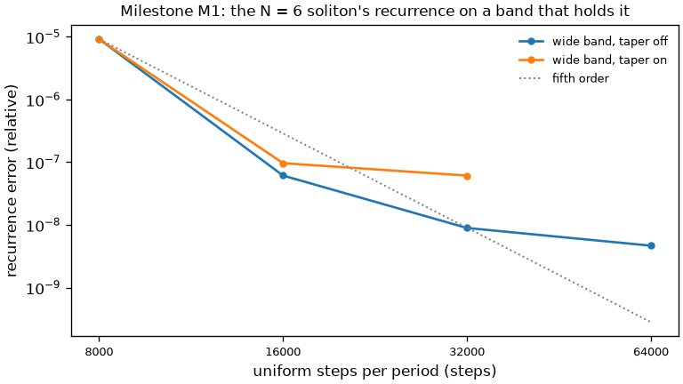
Milestone M1: the N = 6 recurrence error against the step count on the wide band, with the polarisation taper off (the default) and on, from tests/data/convergence/soliton_n6.json (tests/backends/test_numpy_ref_soliton.py). Both ladders leave the scheme’s order and reach a floor; the taper’s is an order higher, because the spectral collar takes the wings off the cubic.#
5. Milestone M2: the RDW example, four modes, 1.5 m gradient#
Convergence order. The case converges at order 1.4–1.5, not five, and the reason is its own: a
fill reaching a true vacuum has dp/dz diverging at the exit. Measured on the reduced
case at 250, 500 and 1000 fixed steps, all four rows run back to back, changing one
thing at a time (coarser rungs exceed the in-stage absorber’s stability limit, 5.5 mm on
this metre, ADR-025). The plasma rows use the held-current source; the Luna comparisons
below run the time-domain gated plasma source through a test-only hook
(tests/gated_source.py):
fill |
plasma |
order |
|---|---|---|
constant |
off |
6.21 |
constant |
on |
5.95 |
vacuum gradient |
off |
1.42 |
vacuum gradient |
on |
1.51 |
The ionisation rate is exactly zero below its threshold and rises steeply above it, which
is the second candidate — and at these rungs it costs nothing: the switch-on is resolved
once the steps are fine enough, and the vacuum end never is, so the diverging dp/dz of
stepper.md section 10, trap 5, is the whole of it. Coarser ladders, at which
the plasma row is not yet asymptotic, attribute the gradient’s cost to the plasma instead.
The answer is converged regardless: two decades of tolerance move the reduced case’s
shape by 6.7e-6 under the default integrator and three decades move the full case’s second-mode exit energy by 2.6e-6
(m2_witness_metrics.json, m2_tolerance.json). Under the per-step split absorber, the
alternative of ADR-025, both move by 2.3e-4: that is the split factor’s own first-order
drift with the step count, not the case’s.
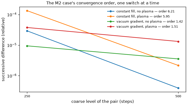
The M2 order study, one switch at a time, from tests/data/convergence/m2_order.json (tests/driver/test_prop_capillary.py). The legend carries each switch’s observed order; the vacuum end is what caps the case, and at these rungs the plasma alone costs nothing.#
Against Luna. The witness is production Luna at rtol = 1e-6, the tolerance its
interface cannot change; a second witness at rtol = 1e-9 is the converged one. All rows
are asserted in tests/driver/test_prop_capillary.py.
metric |
reduced case (2 modes, 1 m) |
|---|---|
fundamental, shape |
5.7e-2 |
fundamental, content |
1.02783 |
VUV band, 100–140 nm |
1.43× in the fundamental, 1.30× over both modes; arrival 4.730 fs against 4.622 fs |
second mode, energy |
1.107 |
The witness runs use the true-power conversion and launch of the introduction; that
launch moves the reduced M2 metrics by parts in 1e4 and not to zero, because the fill is
a gradient, whose change of variables keeps a −½[ln w(z) − ln w(0)] term.
Most of the reduced fundamental’s 5.7e-2 shape is the witness rate’s barrier-suppression
factor, which Luna’s rate lacks: the reduced case run as in
tests/driver/test_prop_capillary.py with that factor alone off — Luna’s own PPT, Stark
shift and dipole factor kept — measures 2.0e-2 and a content of 0.995, and on optmat’s
default helium rate also 2.0e-2. Taking the Stark shift and the dipole factor off as well
raises the shape again to 5.2e-2, so they are not part of the gap.
On the full case the second mode is Luna’s to converge: Luna’s second mode falls from
3.341 to 2.543, 2.101 and 1.893 µJ over rtol 1e-6 to 1e-9 while solprop’s moves by
2.6e-6. With the barrier-suppression correction off the two codes’ on-axis electron
densities agree to 0.04 %, which is what excludes the rate as a cause.
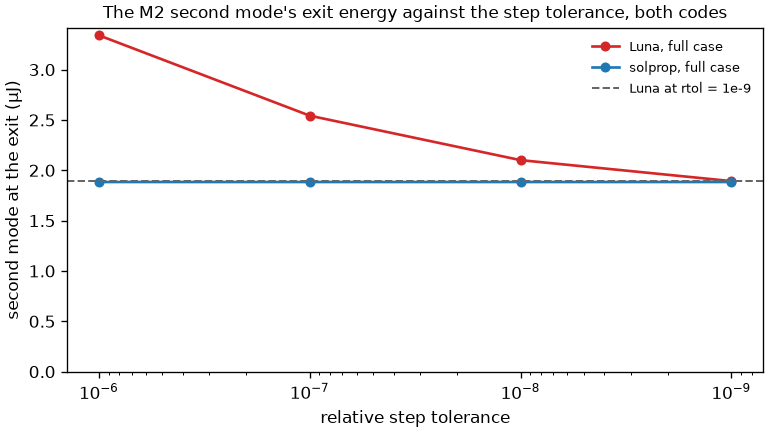
The second mode’s exit energy of the full M2 case against the step tolerance, on both codes, from tests/data/convergence/m2_tolerance.json (tests/driver/test_prop_capillary.py). solprop’s answer does not move across three decades while Luna’s falls by a factor of 1.76 onto it.#
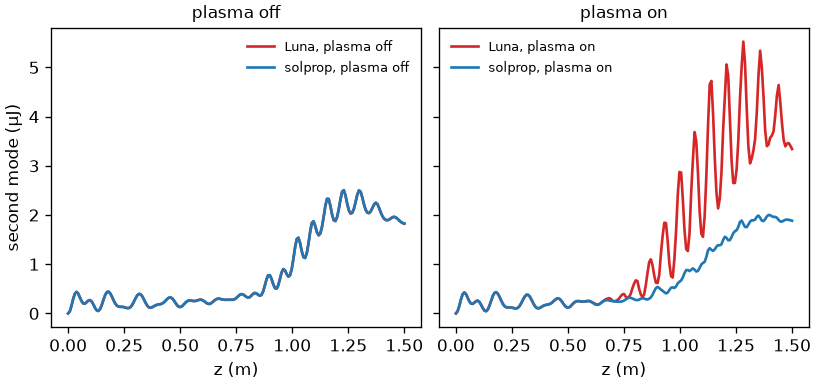
The second mode’s energy along the fibre on both codes, with the plasma off and on, from tests/data/convergence/m2_mode2_along_z.json (tests/driver/test_prop_capillary.py). With the plasma off the two curves lie on each other at every one of 201 planes; with it on the difference is a beat whose envelope departs from about 0.65 m, which is why no z-averaged bound is asserted on it.#
6. Milestone M4: the comb-to-continuum continuum, six modes, 0.2 m#
All rows are asserted in tests/driver/test_prop_capillary.py.
metric |
reduced case (2 modes, 1 ps window) |
|---|---|
input states |
2.014e-6 in total energy, at the 1e-5 pulse/grid bound |
fundamental, shape |
0.15438 |
fundamental, content |
1.04401 |
second mode |
0.58884 |
Stokes rungs, ours over Luna’s |
0.84578, 1.52348, 1.21135 |
peak on-axis field |
0.71 of Luna’s — a single-sample extremum, open, no bound rests on it |
The witness runs use the true-power conversion and launch of the introduction, and match the archived Luna vibrational strength explicitly. The fill is constant, so the change of variables leaves no logarithmic term behind: every metric is within 2e-4 of its vacuum-normalised value, which is the evidence that the launch energy is the whole of the convention’s effect.
The reduced case is a pessimistic one: its window is 2.5 pulse widths and both codes’
collars work there — a twentieth of its input field sits in the temporal collar, so a
change of the collar’s profile moves every metric of the reduced column. The bounds are
±10 % two-sided on the reduced case; numba_cpu reproduces every metric to four figures.
Still open: solprop accepts 11 671 steps to Luna’s 9163 at the same tolerance, a
controller question and not a tuning target.
7. Backend equivalence#
numba_cpu and the installed native backend against numpy_ref, bounds derived from
summation lengths and then measured. No comparison is bitwise
(SEP 25): independent floating-point
computations are compared by numerical error — numpy’s complex multiply contracts into a
fused multiply-add and numba’s does not — so every round-off bound is a multiple of ε. The ladder has two kinds of row, and the criterion follows the kind
(testing.md section 3):
Matched discrete computations: rounding budgets (class R). One application, one step, eight steps, a kernel, a scan, two thread layouts, a batch member or a scan point against the same computation alone: the same method, orders, history, schedule and inputs on both sides. The bound is fixed from operation and reduction counts and transform lengths, with a margin, before anything is measured.
Adaptive runs: accuracy envelopes (class T). A full adaptive run, the reduced M2 and CtC cases, and resumed against uninterrupted runs. Their rows below were derived as rounding budgets and measured while both sides took identical steps, and they stay as the record of what was measured. The criterion is the case’s accuracy envelope against its stored or tighter-tolerance reference: a rounding difference that flips one accept/reject decision, or a different order choice, forks the trajectory, and a forked pair is judged by the envelope, with its step counts a work band rather than an equality.
The device bounds are fixed before any device result: gamma(k) = k ε / (1 − k ε),
Bfft(n) = 512 ε ceil(log2(n)) for one FFT round trip plus its pointwise work, and
Bscan(n) = 192 ε ceil(log2(n)) for the complete deterministic plasma scan chain. CPU
rows keep the bounds below. A CUDA/HIP ladder row uses the larger of that established
bound and its documented number of Bfft envelopes; the analytic family uses
max(1e-13, Bfft(n)). The accelerator record series are named native_cuda and
native_hip, so they cannot overwrite CPU evidence. Reduced M2 and CtC keep their
relative-L2 bounds of 1e-10 and 1e-9.
ladder rung |
bound |
measured |
where |
|---|---|---|---|
one linear application |
32 ε |
4.8e-16 (not bitwise: the contraction above) |
|
one step |
16 ε |
5.0e-17 |
|
eight steps |
128 ε |
2.0e-16 |
|
a full adaptive soliton run |
1600 ε |
6.2e-16 |
|
a capillary with an absorber and a kink |
3200 ε |
1.4e-15 |
|
the analytic field family |
1e-13 |
4.6e-16 |
|
the reduced M2 case |
1e-10 |
3.5e-14, at identical step counts |
|
the reduced M2 case, native CPU |
1e-10 |
3.5e-14, at identical step counts |
|
the reduced CtC field, native CPU against fresh Numba |
1e-9 |
below the bound at identical 1,235 accepted steps |
|
the reduced M2 case, native CUDA |
1e-10 |
5.5534e-13, at identical step counts |
|
the reduced CtC field, native CUDA against fresh Numba |
1e-9 |
below the bound at identical 1,235 accepted steps |
|
native Raman kernel/convolution |
operation-count and FFT-depth bounds fixed before execution |
native host reference, all three drive forms and tail chunks pass |
the native tests under |
the plasma scan’s running sums |
|
2.79e-16 scaled at 256 samples on an x86-64 host; same-path repetition within the same bound |
|
two runs, one thread against many, on one fixed schedule |
the step’s rounding budget from its reduction lengths |
within it |
|
same-backend resume through true-power output |
2.7e-16 of the global field peak; statistic-specific rounding bounds |
field 1.77333e-16; energy up to 2.64009e-16; rate up to 5.06947e-15 |
|
a run continued on the other backend |
— |
2.2–2.7e-16 against either uninterrupted run |
|
The measured columns of the ladder are the committed record. The native CPU and
native_cuda series each cover all seven rungs through reduced M2; on a data-centre
NVIDIA GPU the deviations for rungs 0–5 are 9.56e-22, 7.62e-18, 5.42e-17, 6.10e-16,
9.31e-16 and 2.73e-17 against their device bounds. Raman and CtC equivalence are
separate rows rather than rungs of that ladder.
Polarisation. tests/backends/test_polarised_runs.py extends the ladder with both
polarisation representations at one nonlinear evaluation, one and eight steps, a reduced
adaptive propagation and matching total statistics, for the field-real, field-analytic
and envelope families on NumPy, Numba and native, against a rounding bound derived from
the FFT depth and the two radial reductions before evaluation. Circular plasma has a
separate analytic magnitude/rate/fraction check and a three-resolution
ionisation-energy identity; TE/TM linear fields are checked against their exact
translated operators; the Jones and ellipse helpers have analytic unit tests. The
azimuthal selection tests include an intentionally aliased rule whose forbidden amplitude
must exceed the resolved rule’s bound: a diagnostic control, not a pass of that rule.
Scans and batches are execution paths, not numerical models: a scan point agrees with
the same simulation run alone, and a batch member with the same member run singly under
the same fixed schedule, within a matched-discrete rounding budget, on every backend (scan
points under Local and a fresh Pool; batches of 1, 2 and 3 with a partial final
group). Neither is required to be bitwise: a batch’s lockstep reductions, its thread
layout and a worker process’s library state may order sums differently. A scan point or
batch member run adaptively is class T against its own reference. The short CtC case (0.2 mm, six
modes, three seeds) agrees between native CUDA and numba_cpu to 2.0e-16 relative L2
against the 1e-9 CtC bound, and the reduced M2 case on the GPU with the fixed-schedule
CPU fields to 7.9e-14 (a diagnostic; no bound asserted). A calibrated reduced-M2 schedule
(eight seeds, 515 steps) transfers to 4.7e-7 in its scalar metrics against rtol = 1e-10
adaptive runs, inside the 1e-6 scalar target, but differs by 4.6e-5 in the full field,
which that target does not bound.

Each rung of the backend-equivalence ladder, from tests/data/convergence/backend_equivalence.json (tests/backends/test_numba_cpu.py and tests/driver/test_prop_capillary.py). The bar runs from what the rung measures to the bound derived for it; only the seven rungs of the ladder are drawn, not the separate rows of the table above.#
8. Where Luna is not converged, and where the two codes still differ#
Luna’s weak modes on a stiff case: a factor of 1.76 in the second mode of the M2 case between its default tolerance and a converged one (
rtol = 1e-9); its global weak norm gives a mode at a percent of the fundamental no relative error control, and the tolerance is unsettable through its interface. The quadrature-off control excludes its two first-order mechanisms, the right-endpoint operator and the per-step window, on that case.Accepted-step counts. Luna’s are not reproducible across machines (4856 against 4851 on one case); solprop’s were identical on both when measured, an observation rather than a requirement (SEP 25). solprop takes 27 % more steps than Luna on the CtC case and 58 % fewer on the M2 case at the same nominal tolerance, because the two norms mean different things.
The CtC peak on-axis field, 0.71 of Luna’s on the reduced case; a single-sample extremum, to be recomputed on one definition before it is read as physics.
The spatial witnesses (§10) are diagnostics, not bounds: full Cartesian agreement is close, the modal-prefactor difference explains most of the elliptical-envelope and circular-plasma differences, and radial on-axis and elliptical-field residuals remain.
Not yet measured at all: a Luna comparison above six modes; the mode-2 energy against a converged Luna on the CtC case, which has no converged witness.
9. Regenerating the numbers#
The witnesses. Every Luna witness has a generator beside it under tests/data/
(generate_luna_rdw.py, generate_luna_ctc.py, generate_luna_overlap.py,
generate_luna_rdw_switches.py, generate_luna_rdw_converged.py and the others named
generate_luna_*.py), each recording Luna’s commit, the thread counts and the run time in
its provenance; none is run by the suite, and nothing on this page needs a new Luna run.
The records. Every ladder above writes its rungs to
tests/data/convergence/<study>.json, and every figure above is drawn from one of those
files by docs/dev/accuracy_figures.py. A record holds the study’s name and case, the
axis that varies, one column per metric with its unit, its bound and the tolerance the
column is compared at with the reason for it, the rows, and — per row, not per file — the
commit, machine, backend and thread pools of the run that measured it. Where a Luna
quantity is in a record, the witness it was read out of is named with Luna’s own commit
and the file’s checksum.
The mechanism. tests/convergence_records.py is the mechanism and
tests/convergence_studies.py holds the studies that more than one test file measures
part of. One record(study, request=..., rows=...) call per study test either writes or
compares, and the environment decides which. Rows are merged by (series, axis), so a
study split across tiers accumulates into one file, and provenance is stamped per row: a
default-lane write must not restamp rows a slow-lane run measured at another commit. Each
column carries its bound, rtol, atol and the reason for them in the file, because an
unjustified tolerance is a defect (testing.md section 3) and the tolerance
has to travel with the number. There are two kinds of column, and the difference is the
platform: a scalar quadrature or interpolation ladder is arithmetic that reproduces, and
is compared at 1e-9 with atol at its own round-off floor; a propagation ladder is not —
a different BLAS and a different transform place an adaptive run’s steps differently on
another platform — so it is compared at the width of its own test’s claim. A column may
also be recorded and not compared (rtol of null), which is what accepted step counts
get.
The quoted numbers. The tables and the prose on this page quote numbers by hand, and
a regenerated record does not rewrite them. tests/test_accuracy_page.py lists every
number the page quotes from a record — the passage it stands in, the number as printed,
and the record and row it is read from — and fails when the passage is no longer on the
page or the number differs from the record by more than half a unit in its last printed
digit. When you edit a quoted passage, edit its entry there; when you quote a new number
from a record, add one. The list lives in a test rather than in markup on the page, so
that the page stays plain Markdown. Numbers from the Luna witnesses, from a test’s own
assertion or from a measurement outside the records stay prose, and the test does not see
them.
On every ordinary run each study recomputes its numbers as it always did and compares
them with the stored record; a missing file, a missing rung, a changed case and a number
outside its column’s tolerance are all failures. A record is written only when asked,
with SOLPROP_WRITE_RECORDS=1, and the writer refuses three things outright: a tree that
is dirty outside tests/data/convergence/, because a record that does not match its
commit is not a record; a session under xdist, because several workers would race on
one file; and a CI run. So the lanes never rewrite a record, and a regeneration is
serial.
To regenerate, from a tree that is clean outside tests/data/convergence/, in this
order:
SOLPROP_FFTW_PLAN=estimate SOLPROP_WRITE_RECORDS=1 \
    uv run pytest -p no:randomly

SOLPROP_FFTW_PLAN=estimate SOLPROP_WRITE_RECORDS=1 \
    VECLIB_MAXIMUM_THREADS=1 OPENBLAS_NUM_THREADS=1 OMP_NUM_THREADS=1 \
    uv run pytest -m slow -p no:randomly
then each benchmark-marked writer by hand, per its own docstring — the N = 6 wide-band
ladder at every rung and with the taper on, the two middle switches of the M2 order
study, the full case’s tolerance and quadrature ladders, the second mode along z, and the
two full-size witness comparisons. The environment matters: the thread pins are the slow
lane’s own (poe test-slow) and estimate is the plan flag CI uses, so a record taken
without them is compared in CI against a run that had them.
The spatial records (§10) are written the same way, with an installed native wheel built from the same committed tree:
SOLPROP_WRITE_RECORDS=1 SOLPROP_NATIVE_THREADS=1 OMP_PROC_BIND=false \
    SOLPROP_FFTW_PLAN=estimate uv run --no-sync pytest \
    tests/test_hankel.py tests/test_critical_power.py \
    tests/backends/test_radial_diffraction.py tests/backends/test_radial_absorber.py \
    tests/backends/test_radial_media.py tests/backends/test_radial_nonlinear.py \
    tests/backends/test_radial_statistics.py
A write run is not a green run: it says at the end which files it wrote, and those
are what is committed. And because a stored number is a regression witness, a genuine
improvement fails its comparison — the order is to commit the code with the records
red, regenerate, and commit the records. uv run poe docs-clean before poe docs if a
figure looks stale: the plot directive decides from the page’s own timestamp, not the
record’s.
10. Free space, tabulated, step-index and rectangular modes#
Free-space propagation. The radial tests keep the raw quasi-discrete Hankel transform,
whose exact-orthogonality claim fails at 256 nodes (3.06e-11 against
256 ε = 5.68e-14). The Hankel derivation therefore bounds the
finite-series truncation independently and then adds the special-function construction
and matrix-product rounding; the special-function assumptions and the numerical contour
error estimate are estimates, not interval certificates. spatial_accuracy.json stores
each derived bound beside its measurement and source revision, and every row is held to
two limits: a fixed original limit and the independently derived local bound. The
Gaussian diffraction tests cover the nonparaxial remainder of exact k_z, finite QDHT
bandwidth and radius, the Gouy phase, physical-axis reconstruction and width
interpolation; circular plasma uses an independent electron count and the radial area
measure; absorber refinement is compared against a matrix exponential with a predeclared
Runge–Kutta remainder. The spatial ladders pass on the three CPU backends and on the CUDA build.
Cartesian arithmetic at grazing incidence. At grazing incidence the longitudinal
square \(q = k^2 - k_\perp^2\) approaches zero: a propagating plane wave travels almost
parallel to the transverse plane, and squaring the material and transverse wave numbers in
binary64 loses information before their nearly equal squares are subtracted. Translation
therefore keeps each square’s high part and a residual computed with exact rational
arithmetic from the stored frequency, refractive index and unsquared transverse axes, and
NumPy, Numba and native all evaluate
q = (material_high - transverse_high) + (material_low - transverse_low)
(kernel contract §3); the same correction applies to Cartesian
input pre-propagation. With \(\epsilon = 2^{-52}\),
\(S = |\mathrm{material\_high}| + \mathrm{transverse\_high}\) and \(\eta\) the smallest
binary64 subnormal, the independently derived arithmetic uncertainty of the real
longitudinal square is
derived before any measurement. It treats the stored inputs as exact and does not estimate material-model or experimental uncertainty. The sign of \(q\) is certified where \(|\operatorname{Re} q| > B_q\); a field at an unresolved or exact cutoff is clamped with a warning. Without the split squares, Kerr tests on small Cartesian grids with commensurate grazing bins miss their derivative budgets by seven orders of magnitude, because the rounded square lands on the wrong side of the clamp; with them, every such case meets its budget, and the budgets are not widened for it.
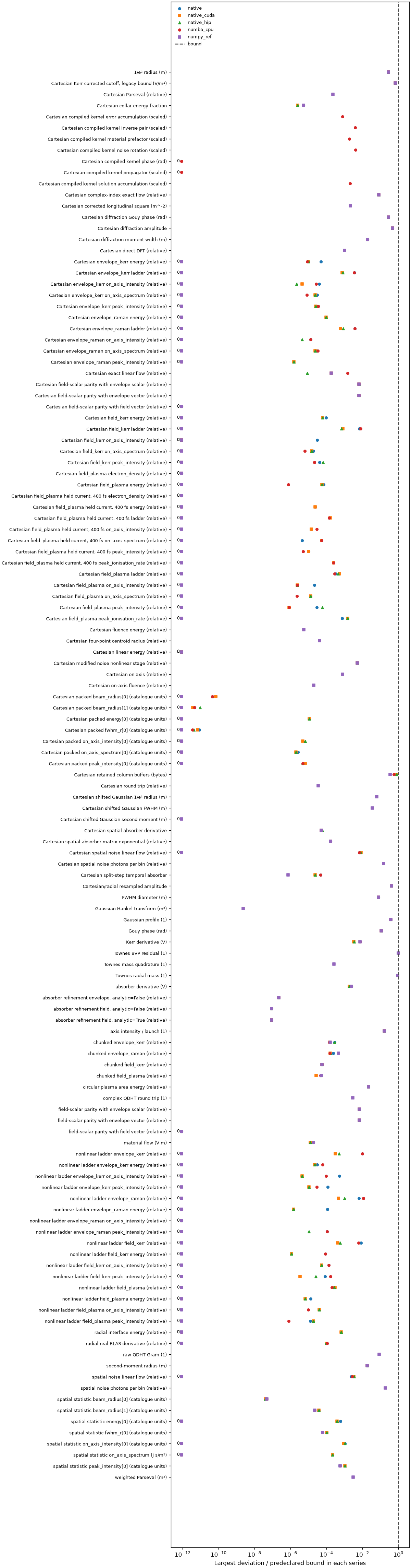
The largest fraction of its derived bound in each spatial series, from tests/data/convergence/spatial_accuracy.json; exact zeros are labelled, and units are in each series name.#
Modes from tabulated data.
comparison |
measured |
evidence |
|---|---|---|
Hollow-table fill rule versus FEM, Kingston argon at 293 K |
max real-index residual 2.24544e-8 on nine smooth rows; 2.82871e-5 near resonance; smooth FEM/table loss 0.99261–0.99843, all away rows 0.85867–0.99843 |
|
50/100/200-knot Marcatili convergence between knots (at the knots, rounding) |
index ratios 15.9766–16.2636; derivative 8.1302–8.3626 |
|
FEM interpolant resolution |
leave-one-out index error 9.15112e-6; raw-row β₂ difference 7.2699 % on the first-band rows above 580 nm (29.5–33.4 nm apart); the vacuum table’s linear imaginary interpolation crosses zero in 20 intervals between 200 and 456 nm |
|
Synthetic GNLSE table versus Taylor field |
relative amplitude error 8.88294e-8; operator-derived bound 3.93114e-5 |
|
These are one-fibre witnesses and numerical integration checks.
Step-index and rectangular modes.
check |
measured |
bound / interpretation |
|---|---|---|
40-digit step-index index witness |
2.22e-16 relative |
1e-13 |
Implicit derivative witness |
8.82e-14 relative |
1e-12 |
Richardson derivative |
1.10e-11 relative |
1e-9 |
HE11 parity Gram, 24 radial nodes per panel |
6.66e-16 |
1e-12 |
HE11/HE12 adaptive electric-field overlap, delta = 0.005/0.05 |
2.536e-4 / 3.026e-3 |
exceeds the unchanged 1e-6 multimode gate |
Matched-material rectangular Luna witness |
2.23e-16 relative |
1e-15 rounding |
Four rectangular modes, Gram |
2.55e-15 |
1e-12 |
Rectangular (3,2) quartic, per axis |
22 nodes give 1.99e-13; 20 give 6.8e-11 |
1e-12; shipped rule |
Rectangular refractivity against mpmath, 10 cm guide |
2.02e-16 relative |
4 ε; the naive spellings are 5.63e-6 |
Metal complex index versus Luna, Ag/Al |
29.4002 % / 7.75281 % |
source and interpolation differences, not accuracy |
Metal-wall rectangular derivative against Richardson |
4.67e-12 (x) / 4.33e-12 (y) |
2e-11; the C2 spline’s fourth derivative limits it |
Step-index cladding-slope derivative against Richardson |
3.36e-11 (NA core) / 1.06e-10 (constant core) |
1e-10 / 4e-10 |
|
6.43e-12 of the peak field |
128·8·n_t·ε = 2.33e-10 |
A user’s 400-knot table of the same fibre |
4.67e-5 of the peak field |
1e-4; from a 7.05e-10 index interpolation error |
The silica strand’s GVD at 835 nm is −11827.1342 fs²/m and its ZDW is 780.31945 nm. Rectangular FEM-checked Luna values keep their 1 % loss and 1 nm ZDW bounds; Luna’s committed 210 nm constant is itself 0.135 % from its own present table.
11. Capillary modes, Raman and the moving basis#
The capillary derivative. The analytic \(dn_{\rm eff}/d\omega\) of
MarcatiliMode is checked against three independent
references, because an analytic derivative is exactly the kind of thing that is nearly
right (tests/modes/test_capillary.py):
A contour integral. \(n_{\rm eff}(\omega)\) is holomorphic, so Cauchy’s formula on a circle in the complex frequency plane, sampled by a trapezoid rule, gives the derivative with no subtractive cancellation. It pins the result to about \(10^{-12}\) relative (the gate is \(10^{-11}\)) — three orders better than any finite difference of the same function. The circle wants to be large: the trapezoid rule’s truncation falls like the radius to the power of the node count, while the rounding it amplifies grows as one over the radius.
A symbolic derivation.
tests/data/generate_symbolic_marcatili.pydifferentiates the closed-form index with sympy, for the full and the reduced model and with and without loss; \(\beta\) and \(\beta_1\) agree with it to \(2\times10^{-16}\).Finite differences at three step sizes, which mostly show that the finite difference is the limited party: the best a central difference can do is about \(10^{-6}\) relative, because \(n_{\rm eff}\) is 1 plus a small number and the rounding is relative to the 1.
\(\beta_2\) is the one quantity solprop differences: the second derivative of a gas
susceptibility is not part of the material interface, so
beta2() is a Richardson difference of the analytic \(\beta_1\).
One derivative differenced instead of two, it reaches about \(5\times10^{-9}\) against the
symbolic result (asserted at \(10^{-7}\)), where a second difference of \(\beta\) itself
reaches only about \(10^{-6}\).
Sampling a capillary along its length. Position enters the effective index through
exactly two scalars, \(a(z)\) and \(\rho(z)\); everything frequency-dependent is sampled once
as MarcatiliTerms, so the Chebyshev builder can
evaluate the operator at hundreds of positions for two scalars each:
terms = mode.sampled_terms(omega)  # the expensive part, once
index = mode.neff_from_terms(terms, radius, density)  # per position, cheap
The factorised path regroups the direct evaluation’s roundings and is held to it within
the one-evaluation budget of 16 ε (§7), normwise, at three positions of a gradient
(tests/modes/test_capillary.py).
The Raman response. The numerical checks of the
Raman response, in
tests/backends/test_numpy_ref_raman.py. Their measured errors apply to the stated
configurations and are not a general error bound for a new simulation.
claim |
how it is checked |
measured |
|---|---|---|
the pass is the oracle |
given the oracle’s own kernel, on both grids for N₂, H₂ and SiO₂, |
within one convolution’s rounding, |
the backend’s damped spectrum is the translation layer’s |
against |
within the same bound; exactly zero at zero density |
what a run convolves with, against the oracle |
the grid-collar taper of the kernel’s tail is the only difference |
within rounding for a glass on a window that holds its response; 12 % for hydrogen on a 228 fs window, whose rotational coherence outlives it by four orders of magnitude |
\(\mathrm{Im}\,\tilde H\) is the line |
against the Lorentzian \(-Ka/(2(a^2+\delta^2))\) of nitrogen’s 69.85 THz vibration |
1.00000 |
the small-signal gain |
the Stokes growth rate against \(\kappa\,\tfrac23(-\mathrm{Im}\,\tilde H)/\chi^{(3)}\), with \(\kappa\) the pump’s own Kerr phase rate, so the normalisation cancels |
0.4 % on a 140 ps window, 1.6 % on 70 ps |
the soliton self-frequency shift |
the centroid rate against Gordon’s $-8 |
\beta_2 |
photon number |
$\sum |
A(\omega) |
The gain and the shift are stated against the run’s own quantities on purpose: the kernel spectrum is what the convolution multiplies by, and the first moment of the silica shape is what \(T_R\) is. What is closed-form about them is the chain in between — the factor of a half in the drive, the three quarters in the envelope cubic, the sign of the imaginary part and the normalisation prefactor — and that chain is what the ratios test.
The connection of a moving basis. The
moving modal basis carries the connection
\(\Gamma = W^{-1}S\) of a guide whose modes change along z
(tests/modes/test_modal_connection.py). Its reported antisymmetry is the residual of
the metric identity with \(W'\) differenced independently of the pairing, so it is a
statement about the sampling and not about the arithmetic; it is admitted below \(10^{-8}\)
of the connection’s own scale (measured \(7.4\times10^{-11}\) on a step-index taper and
\(5.7\times10^{-9}\) on a graded-index one). Two independent references check it:
A step-index core’s \(HE_{1m}\) fields become the Dirichlet Bessel set as \(V\) grows, and that set is the one the capillary’s connection was derived on, so this connection must approach that closed form. It does, and the departure halves as \(V\) doubles — 4.6 % at \(V = 20\), 1.5 % at 56, 0.34 % at 223 — which is the Goos–Hänchen penetration depth’s own \(1/V\). At a finite \(V\) the two are genuinely different, which is why the connection is derived rather than transplanted.
A physical field frozen at the entrance and propagated on the connection alone matches the coefficients the same field has on the exit basis by direct projection to second order in the total contraction; propagating with \(+\Gamma\) instead is two orders worse, which is what fixes the sign.
For a declared z-dependent unitary change of basis, dropping the connection term moves the propagated state by at least a fifth of its own size in the test case, while keeping it reproduces the direct propagation to \(10^{-10}\) of the state. That is a measurement for that comparison, not a general estimate for a changing basis.
12. Coupling between simulations#
A coupling (SEP 31, the manual’s chapter) joins two runs that each have their own accuracy envelope; the coupling adds its own, and the three are kept apart rather than folded into one number.
The source and the receiver are ordinary runs: their step-control and discretisation envelopes are those of their routes (§1 to §11). A coupling takes the source plane as stored and makes no claim about it. A source run through a gas gradient carries SEP 34’s adiabatic path certificate, which the coupling report and the transport report carry separately (
report.certificate,report.source_certificate): it bounds the linear background path, not the coupling.The coupling model’s error is the
model_errorbudget \(\epsilon_m\) and the admission items that must fit inside it: the angular cone rule (an allocation \((1-\cos\theta_*)\) of the cone share, plus the measured tail), the metric defects between the common measure and each native metric, the H-closure of the vector model, the passive-map certificate and the recorded pair envelope. The envelopes are measured against independent physics, not the model’s own profiles: the capillary’s against Marcatili’s leaky core field \(J_0(u_m(1 - i\delta)r/a)\), \(\delta = |\nu_n|c/(\omega a)\) (largest share discrepancy \(2.9\times10^{-3}\) at \(\delta = 10^{-2}\) over its range, bound \(6\times10^{-3}\), scaled linearly by the pair’s energy-weighted \(\delta\): about \(1.5\times10^{-3}\) for a 75 µm silica capillary at 800 nm); the step-index pair’s against the exact vector \(HE_{11}\) flux overlap (\(3.0\times10^{-4}\)). Bins outside an envelope’s range are counted in full.The coupling’s numerical error is its own item: the source plane’s content at its spectral edge, an analytic field’s domain and resolution checks (the energy change on doubling the window and halving the spacing), and the overlap quadrature (its amplitude error \(\delta\) entered as \(2\delta + \delta^2\)). Representation errors of a synthesised exit (
Outcouple.window) and a transport’s thin-screen and Fresnel bounds are reported by those operations.
Refinement is separate for each: a quadrature is refined by halving its panels, a
plane’s domain and resolution independently, the captured subspace by nested mode sets
(which share their common shares to \(10^{-12}\) on the capillary tests), and the
propagation by the receiving run’s own tolerance. A launch is never renormalised, so an
error in any one of them appears as an energy discrepancy in the report rather than
being hidden by rescaling to the requested energy. The integrated compositions of SEP
31 §2 (tests/coupling/test_workflows.py) assert the ledger of each: incident equals
captured plus uncaptured, the launch differs from the captured energy only by the
reported target-metric defect, and the receiving run’s entrance carries exactly the
launch.