The kernel problem#

Before a run takes its first step, everything solprop knows about it — the grid, the modes, the gas, the frame, the responses, the pulse, the noise, the stepper settings — is translated once into a single frozen object of plain NumPy arrays, a KernelProblem. That object is the only thing a backend ever sees, so it is exactly what the run computes: every choice the physics pages describe has been made by the time it exists, and nothing a backend does can change them.

You rarely need to handle it, but it is the place to look when you want to know what a run will actually do. Simulation.translate builds it (once; the result is cached) and returns it:

from solprop.driver import Simulation

simulation = Simulation.from_gnlse(
    0.11,
    0.01,
    [0.0, 0.0, -1.183e-26],
    lambda0=835e-9,
    wavelength_limits=(500e-9, 2e-6),
    trange=1e-12,
    width=100e-15,
    peak_power=9.8,
    pulseshape="sech",
    n_save=3,
)
problem = simulation.translate()
problem.shape  # (1, 1, 1, 1024): batch, modes, polarisation, frequency
problem.flags  # single_mode=True, constant_linop=True, ...
problem.linear.phi_representation  # 'constant': how the linear operator was stored

This page explains what the problem holds and where the physics ended up in it, for a reader who wants to understand or check a run. Its field-by-field specification, for anyone writing a backend, is the kernel contract; why the line between the physics and the backends is drawn here is in the architecture notes, §3, and the backend notes. In short, a backend exists to change the structure of the computation — to fuse passes, to reuse buffers, to keep transforms in place — so the seam is drawn at the level of operations on the propagated state, and everything on the physics side of it is compiled away beforehand.

What crosses#

solprop.translate.problem.KernelProblem is built by solprop.translate.problem.assemble() and carries eight groups, one per section of the contract:

group	holds
`flags`	static booleans and channel/response counts for kernel specialisation
`grids`	the frequency axis, the two band masks, the windows, the crop index and the two oversampling scale factors
`linear`	the cumulative operator \(\Phi(\omega, z)\) as a Chebyshev expansion in the mode set’s scalar paths, or as a table along z where that is not available, plus its hard kinks and the frame quantities
`transform`	synthesis and projection between modal amplitudes and the field at quadrature nodes, and their rescaling along z
`responses`	the compiled nonlinear term: the Kerr coefficients, the ionisation table, the plasma and Raman leaves, the density path, the prefactor, the temporal absorber
`initial`	the initial state, the noise realisation and the per-member batch parameters
`stepper`	the tableau, the controller, the step caps, the save planes and any fixed schedule
`stats_spec`	which statistics to collect
`flux`	a spatial run’s plane measure: the axial admittance of the medium at any plane, from which every spatial statistic is weighted (SEP 34, version 35)

Every array is float64, complex128, bool or intp (and int32 at three named index leaves of the general modal route); C-contiguous; read-only; and in the FFT convention with the phase origin at the first time sample (the conventions, §2). The user’s optics-convention inputs were converted by the pulse builders and the observations are converted back by the output layer; no backend ever conjugates anything.

Nothing that is not an array or a number crosses. A ZProfile is a Python object with a __call__, which a compiled loop cannot use, so anything that varies along z — the gas density, the effective area, a taper’s rescaling, the frame quantities — becomes a scalar-valued PiecewiseChebyshev over the same range as \(\Phi\), evaluated by one Clenshaw pass on the host.

The two array-valued things that vary along z, \(\Phi\) and the prefactor, are carried the same way as each other: constants, parameter expansions, z tables, or the separable constant-media spatial representation. Both are functions of the scalar paths rather than of the position — a Marcatili mode reaches z only through its core radius and its number density — so both are expanded in those parameters, with scalar tables along z (the expansion in the parameters). Where that is not available they fall back to a Chebyshev table of z. The NumPy reference evaluates through delta_phi(), unitary_phase() and prefactor_at(). Compiled backends combine fixed terms with the small host-scalar stage bundle. Numba CPU also evaluates z tables through its host adapter, and native’s CPU build evaluates them natively into term slots that the stage weights select; its device builds refuse them. See the kernel contract for the spatial representation and exact support rules.

Where the normalisations live#

The nonlinear term is a chain of scalings, and the contract has to say which link carries each of them. Two are worth stating here because the natural guess is wrong.

The oversampling pad scale \(n_{to}/n_t\), which makes the fine and coarse time samples agree where they coincide, is folded into transform.synthesis — not into a response coefficient. A coefficient can absorb a field scale only when the response is homogeneous in the field. The Kerr term is; an ionisation rate, which is a table looked up at the physical field amplitude in volts per metre, emphatically is not. Folding the pad into the synthesis means every response sees the physical field, whatever its degree.

The crop scale on the way back has no such condition, so it is folded into responses.prefactor, which is applied in the same pass as the crop. The prefactor is the UPPE factor \(-\mathrm{i}\omega / (2\varepsilon_0 c\, \mathrm{Re}\, n_\text{eff})\), or its mode-averaged composition with the effective-area conversion, and it is exactly zero outside the active band rather than one: raw, unnormalised polarisation left in the out-of-band bins would be seen by every Runge–Kutta stage and every error estimate.

The prefactor follows z, and its two halves are carried in different places. The effective area is carried by transform.taper_scale, which rescales the synthesis and divides the projection; so the prefactor holds the area at the reference position and lets only \(\mathrm{Re}\,n_\text{eff}(\omega, z)\) vary, because carrying the area here as well would count it one and a half times on a taper. What the two supply together is the full mode-averaged prefactor at every position:

\[ p(\omega, z)\;/\;\tau(z) \;=\; \text{mode\_average\_prefactor}(\omega, z) \times \text{crop\_scale}, \]

an identity the tests hold to \(7\times10^{-16}\). On a fill, where the bore does not move, the prefactor simply is the mode-averaged one.

Carrying it costs almost nothing, and freezing it at the entrance would discard a relative swing of \(2.5\times10^{-4}\) on a gradient capillary (1.5 m of helium falling from 5 bar to 0.1 bar), and more on a glass taper. As a table on that capillary it needs 9 intervals of degree 32 and 9.3 MB, because the mode set’s scalar paths are resolved before the table is built (7 intervals of degree 63 and 14 MB without that, at the same accuracy); as an expansion it is 10 terms and less of everything. Either representation reproduces direct evaluation to \(5.5\times10^{-15}\) at twenty random positions. Unlike \(\Phi\), the prefactor needs no relaxed tolerance: its relative round-off is \(8\times10^{-16}\) against the operator’s \(10^{-11}\), because nothing in it cancels the way the co-moving frame cancels eight digits out of \(\beta\). One Clenshaw pass per stage evaluates it, where Luna’s norm_mode_average recomputes \(\beta(z)\) over the whole active band at every stage. A mode set that does not vary along \(z\) skips the pass entirely: responses.prefactor_constant holds the array, exactly as linear.phi_constant does for the operator.

The flags are derived, never declared#

The ten booleans of section 1 — single_mode, has_raman, constant_linop and the rest — are computed by solprop.translate.problem.Flags.from_content() from the arrays that were actually built. A caller cannot set them, so a flag cannot disagree with what it describes, which is the failure mode a kernel specialising on them would find hardest to debug.

Validation is the backend’s defence#

A backend calls solprop.translate.problem.KernelProblem.validate() and refuses anything inconsistent. Most of the contract’s promises are kept by construction — each group freezes and checks its own arrays, so a writeable array or a mismatched interval count cannot be built in the first place — and what validate adds is everything that spans groups: the schema version; the shapes against the canonical state shape; finiteness; that the \(\Phi\) table covers the run; that every table along z spans the same range; and that a replayed fixed schedule lands on every save plane and every hard kink. A failure raises solprop.exceptions.TranslationError naming the field.

What is compiled#

The instantaneous Kerr response, the delayed Raman response and the plasma response compile, each into its own leaf of responses, and responses.response_order lists the passes a stage makes, in order.

Plasma. A plasma carries its own ionisation rate, so it supplies the run’s ionisation_table tuple and, beside it, one labelled PlasmaChannel per ionising population (each species of a gas mixture is one): the two constants of its currents, its number-density and pre-ionised-fraction paths along z, and the rate table it reads. Each channel scans its own ionisation fraction in time; their weighted free-electron currents and ionisation losses are then summed and integrated together (strong-field ionisation). A plasma adds the passes intensity, ionisation_rate, plasma_scan, plasma_current to response_order, before kerr.

Raman. Each Raman component fills one member of the raman_terms tuple (the contract’s §5) — the undamped model responses on the doubled grid, one decay-rate table per row, the fraction, and the drive form — and adds raman_drive to response_order after kerr (sampling the kernel). It is refused on a problem with two polarisation components unless every term has an established vector contraction (tensor_capable: none is declared scalar_only), and on a field grid it is refused without a Kerr response beside it, or beside one that disagrees about thg: whether the drive keeps the \(2\omega\) beat is a property of the problem, which is why the two must agree and why the answer is a field of the leaf rather than a property of either response.

Envelope plasma. The cycle-averaged plasma of an envelope grid (envelope plasma) compiles into a spectral assembly of three streams — the ordinary polarisation, the Drude drive and the loss current — which stay separate through the spatial projection and the forward temporal transforms and are combined, each with its own frequency factor on the coarse axis, just before the UPPE prefactor. Any other response that needs a spectral assembly of this kind is refused by name. The real-field PlasmaResponse refuses an envelope grid; declare EnvelopePlasmaResponse for the cycle-averaged route.

The transverse components belong to one axis. A row of transform.synthesis is one Cartesian component at one quadrature node, and so is one entry of the state’s polarisation axis, so a problem carries them in the transform or in the state and never in both; assemble and validate both refuse the combination. Which components a multimode transform resolves is the components keyword of assemble(), defaulting to DEFAULT_COMPONENTS — the direction an \(\mathrm{HE}_{1m}\) mode points at \(\phi = 0\), which is \(x\) (polarisation).

A worked example#

A fundamental-soliton problem, assembled by hand for a kernel: a dispersion-specified fibre, so the operator does not vary along z and the table is the exact one-interval fast path, and the compiled prefactor that carries the crop scale and the band mask.

import matplotlib.pyplot as plt
import numpy as np

from solprop.grid import EnvelopeGrid
from solprop.nonlinear.gnlse import problem_from
from solprop.pulses import SechPulse
from solprop.stepper import PIController
from solprop.translate.problem import assemble

grid = EnvelopeGrid.from_limits(1.0, 835e-9, (500e-9, 2e-6), 4e-12)
gnlse = problem_from(
    [0.0, 0.0, -11.83e-27], omega_ref=grid.omega0, gamma=0.11, shock=False
)
peak = 11.83e-27 / (0.11 * 100e-15 ** 2)      # the fundamental soliton, 10.75 W
start = SechPulse(wavelength=835e-9, width=100e-15, peak_power=peak).build(grid)

problem = assemble(
    grid, gnlse.mode, [gnlse.kerr], start,
    controller=PIController(rtol=1e-8, atol=1e-14),
    save_planes=[0.5, 1.0], dz_max=0.05, dz_init=1e-4,
    density=1.0, shock=False, prefactor_index=1.0,
)

omega = problem.grids.omega
order = np.argsort(omega)
detuning = 1e-12 * (omega[order] - problem.grids.omega0) / (2 * np.pi)
# A dispersion-specified fibre does not vary along z, so the prefactor is the array
# of the fast path rather than a Clenshaw pass over its table.
prefactor = np.abs(problem.responses.prefactor_constant[0, 0])[order]
operator = problem.linear.phi_constant[0, 0, 0][order]

fig, (left, right) = plt.subplots(1, 2, figsize=(7.0, 3.0), layout="constrained")
left.plot(detuning, -np.imag(operator), lw=1.6, color="C0")
left.set_xlabel(r"$(\omega - \omega_0)/2\pi$  (THz)")
left.set_ylabel(r"$-\mathrm{Im}\,D$  (1/m)")
left.set_title("the operator inside $\\Phi$")

right.plot(detuning, prefactor, lw=1.6, color="C1")
right.set_xlabel(r"$(\omega - \omega_0)/2\pi$  (THz)")
right.set_ylabel(r"$|p(\omega)|$  (m/(V s))")
right.set_title("the compiled prefactor")

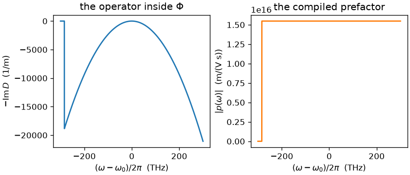
Both are exactly zero outside the active band, which is the whole of the band limiting the kernel has to do: the operator does not propagate what is not there, and the prefactor does not create it. Between the two, the assembled problem reports

shape          (1, 1, 1, 4096)
grid_kind      'envelope'
flags          single_mode, scalar_pol, single_batch, constant_linop, mode_averaged
Phi table      1 interval of degree 1, 128 kB
save planes    [0.5, 1.0]

and a backend built on it needs to know nothing else.

Rebuilding, and the schema version#

When a mixture is updated — in a scan over fill fractions, say (with_mixture()) — the rebuild carries a host-side TranslationReuse record. It shares the initial field and the transverse transform, the immutable rate tables and the undamped Raman samples that did not change. The previous build’s expansion terms are kept only when the sampled operator function and the parameter ranges still cover the new paths; changing the fill fractions invalidates a pressure expansion. Scalar weights and material tables are rebuilt. The record stays on the host and never crosses to the backend.

The problem carries a schema version, which every backend checks before it runs one; a saved output file carries its own, independent metadata schema. The current numbers are stated at the top of the kernel contract.