Envelope plasma: model, derivation and limits#
Solprop’s envelope plasma model follows the electron population, its collisionless acceleration and the optical energy spent on ionisation. It supports a scalar envelope or two Cartesian polarisation components. The model solprop uses is frozen-cycle averaging of an instantaneous isotropic ionisation law, with the first harmonic of the vector ionisation-loss current. This chapter explains what that choice means physically, how it relates to the literature, and what the numerical qualification establishes.
The chapter is for readers who run ionising pulses on an envelope grid and want to
know what the plasma terms represent, when they can be trusted, and why the
alternatives in the literature are not used. To turn the model on and read its output,
go straight to section 10: in short,
envelope=True, plasma=True on prop_capillary or prop_waveguide. Constructor
examples and rate options are in
strong-field ionisation, and the
carrier/envelope tutorial
compares a complete envelope run with a carrier-resolved one. The field-grid plasma
response it is compared against is on nonlinear responses.
1. Three separate choices make a plasma model#
An ionisation formula alone does not specify how to propagate a pulse through the resulting plasma. Three pieces must agree:
Ionisation rate: how often an available atom or molecule releases an electron. In this implementation it is a scalar function \(W(|\mathbf E|)\).
Current and energy accounting: how existing electrons accelerate, and how the electromagnetic field supplies the binding energy of new electrons.
Optical representation: whether to resolve the real carrier field or retain only its slowly varying complex fundamental envelope.
Geissler, ADK and PPT therefore name different parts of the calculation. The following table gives their roles, including alternatives that were compared and not implemented.
Model or source |
What it supplies |
Role in this implementation |
|---|---|---|
Geissler et al. (1999), Eqs. (4)–(6) |
Collisionless acceleration, population depletion and ionisation work for a real, linearly polarised field |
Starting point for the current closure; extended to an isotropic Cartesian vector field and then averaged |
ADK, PPT and molecular ADK |
Quasistatic tunnelling and the multiphoton-to-tunnelling rate for linear polarisation, atomic and orientation-averaged molecular |
The theories behind optmat’s curated rate models, which |
Gulley–Dennis (2010) |
An envelope derivation distinguishing free current from ordinary polarisation |
A cross-check on the inverse-frequency factors; its collisional terms are outside this model |
Elliptic PPT and Popov’s review |
Nonadiabatic action, polarisation dependence, asymptotic regimes and Coulomb corrections |
Research comparisons; no elliptic atomic rate is implemented |
Barth–Smirnova circular theory |
Orbital-resolved circular ionisation, including different co- and counter-rotating p-orbital rates |
A separate research comparator that exposes physics absent from an isotropic magnitude law |
Yudin–Ivanov (2001) |
Ionisation with explicit subcycle phase dependence |
A research comparator requiring a different rate interface and a separately derived current closure |
The choice preserves a consistent rate–population–current combination and gives continuous scalar, linear, elliptical and circular limits. It also lets the carrier-resolved implementation act as an independent comparison using the same physical rate law. Such a comparison measures the envelope approximation; it does not measure the accuracy of that rate against an atom.
2. Fields, densities and normalisation#
This chapter uses the optics convention
The internal FFT convention is its conjugate, as specified in conventions. The distinction changes spectral signs; it does not change a population, an intensity or an energy.
Symbol |
Meaning |
Units |
|---|---|---|
\(\mathbf a\) |
Physical complex electric-field envelope |
V/m |
\(A_m\) |
Propagated modal amplitude |
\(\sqrt{\mathrm W}\) |
\(\rho_s\) |
Available single-ionisation sites in species channel \(s\) |
m⁻³ |
\(f_s\), \(s_s=1-f_s\) |
Ionised and surviving fractions |
dimensionless |
\(n_{e,s}=\rho_s f_s\) |
Electron density produced by that channel |
m⁻³ |
\(I_{p,s}\) |
Binding energy paid per newly released electron |
J |
\(\mathbf d_D\) |
Time derivative of the Drude current, before carrier removal is accounted for |
A m⁻² s⁻¹ |
\(\mathbf j_L\) |
Fundamental envelope of the ionisation-loss current |
A m⁻² |
\(\mathbf p\) |
Equivalent polarisation envelope |
C/m² |
At a fixed propagation position, \(\rho_s\) is fixed during the temporal population scan. A longitudinal density profile may change it at the next position. The remaining neutral density is \(\rho_s s_s\), rather than \(\rho_s\) itself. None of these densities is the optical mode index \(n_{\mathrm{eff}}\).
For a mode-averaged calculation, \(\mathbf a=\sqrt{2/(\varepsilon_0 c A_{\mathrm{eff}})}\,\mathbf A\). For a resolved modal calculation, the real mode profiles give \(\mathbf a(\mathbf x,t)=\sum_m A_m(t)\mathbf e_m(\mathbf x)/\sqrt{N_m}\), where \(N_m=(\varepsilon_0c/2)\int|\mathbf e_m|^2dA\). Radial and Cartesian calculations evaluate the response on the local physical V/m field and keep their own transverse-transform normalisations. The rate is evaluated on that physical field, never on a modal amplitude in \(\sqrt{\mathrm W}\).
3. From the Geissler current to an envelope#
Acceleration and ionisation work#
In the single-ionisation model, the real-field population obeys
The collisionless Drude current and the isotropic ionisation-loss current are
These are SI current densities. The factor \(e^2/m_e\) has no inverse permittivity; \(\varepsilon_0\) enters the Maxwell propagation prefactor. At zero field the loss is defined by the vanishing-rate limit of the accepted magnitude law. The rate/table threshold makes that limit explicit in computation.
The acceleration equation assumes electrons are born with zero mean velocity and any initially present electrons have zero initial mean current. Summing the contribution of every birth time gives
There is no additional birth-velocity source under that assumption. A theory with nonzero exit momentum must revisit it. The choice of \(\mathbf J_L\) along the instantaneous real field is the isotropic closure used here. Its work is
Thus it removes one binding energy per new electron. The work identity alone would not determine arbitrary transverse components of a vector current; the collinearity assumption is part of the model. This is the Cartesian extension of Geissler et al., Eq. (4), whose original derivation is for linear polarisation.
Freeze a cycle, retain its fundamental#
At each envelope time sample, freeze \(\mathbf a\) and the slowly varying neutral survival \(s\). Let \(\theta\) run around one optical cycle:
The averaged rate and the retained loss-current envelope are
The factor two reconstructs a real signal from the complex amplitude of its positive-frequency fundamental. This operation retains the fundamental current and discards its higher optical harmonics. The Drude drive becomes \(\mathbf d_D=(e^2/m_e)\rho f\mathbf a\), with \((\partial_t-i\omega_0)\mathbf j_D=\mathbf d_D\).
Freezing the survival within a cycle is an approximation. It removes the subcycle correlation between electron births and the optical field. Accurate angular quadrature cannot restore that correlation when depletion in one cycle is substantial.
4. Why ellipticity needs two loss moments#
Write \(\mathbf a=\mathbf x+i\mathbf y\) with real Cartesian vectors. The polarisation ellipse has semiaxes \(u\ge v\ge0\), determined by
Here \(I\) is a field-squared invariant, not intensity in W/m². In the package’s field normalisation the corresponding intensity is \(\varepsilon_0cI/2\). After a real Cartesian rotation and a common phase shift, the envelope can be written \((u,iv)\). Reversing handedness conjugates it. For \(u>0\), define \(q=v/u\), \(d(\theta)=\cos^2\theta+q^2\sin^2\theta\) and
Then, in principal-axis coordinates,
The two moments weight different parts of the cycle. A single scalar attenuation coefficient multiplying \(\mathbf a\) generally loses that information. The implementation reconstructs the Cartesian current from the real Gram matrix \([\mathbf x\ \mathbf y]^T[\mathbf x\ \mathbf y]\), using scaled components to avoid overflow and cancellation near a degenerate ellipse.
The limits have direct physical interpretations:
Linear, \(q=0\): the minor-axis current vanishes; the rate samples the field from zero to the major-axis peak. The scalar result is recovered.
Circular, \(q=1\): the real-field magnitude is constant, so \(\overline W=W(u)\) and \(M_c=M_s=W(u)/2\). No preferred ellipse angle exists.
Zero field: rate, new ionisation and both sources vanish. A previously created population can remain, but it has no drive without a field.
Common phase or real Cartesian rotation: population is invariant and the current transforms with the envelope. A general complex change of polarisation is not a symmetry: it can change ellipticity and therefore the rate.
An analytic counterexample to a scalar loss coefficient#
Use the dimensionless test law \(W(E)=E^4\), solely as an algebraic oracle. Direct integration gives
For \((u,v)=(2,0.7)\), the current is \((6.245,0.95725i)\) and the cycle work is \(6.5800375\) in these test units. The collinear choice \(\mathbf j_L/(I_p\rho s)=2\overline W\mathbf a/I\) has exactly the same work but differs by about 18.35% in vector norm. Passing an energy test alone would therefore miss a wrong vector response.
import numpy as np
import matplotlib.pyplot as plt

phase = np.linspace(0, 2 * np.pi, 401)
fig, axes = plt.subplots(1, 2, figsize=(9, 3.4))
for q, label in [(0, "linear"), (0.35, "elliptical"), (1, "circular")]:
    magnitude = np.sqrt((np.cos(phase)**2 + q*q*np.sin(phase)**2) / (1 + q*q))
    axes[0].plot(phase / np.pi, magnitude, label=label)
axes[0].set(xlabel="optical phase / pi", ylabel="field magnitude / sqrt(I)")
axes[0].legend(frameon=False)
u, v = 2.0, 0.7
mean_rate = (3*u**4 + 2*u*u*v*v + 3*v**4) / 8
directional = np.array([3*u*u + v*v, u*u + 3*v*v]) / 4
collinear = 2 * mean_rate / (u*u + v*v)
positions = np.arange(2)
axes[1].bar(positions - 0.18, directional, width=0.36, label="two moments")
axes[1].bar(positions + 0.18, [collinear, collinear], width=0.36, label="scalar coefficient")
axes[1].set_xticks(positions, ["major axis", "minor axis"])
axes[1].set_ylabel("loss coefficient / (Ip rho s), test units")
axes[1].set_ylim(0, 4.3)
axes[1].legend(frameon=False)
fig.tight_layout()
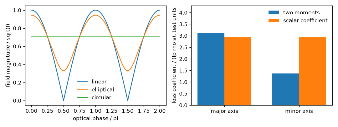
A dimensionless polynomial example, not an atomic-rate prediction. Left: changing ellipticity changes the field magnitude during a cycle even at fixed total intensity. Right: the two loss moments give different attenuation along the principal axes; a scalar coefficient matches their weighted work but not both components.#
Comparisons of polarisation must also say what is held fixed. At fixed major axis use \((F,iqF)\); the total intensity then grows with \(1+q^2\). At fixed intensity use \((F,iqF)/\sqrt{1+q^2}\); circular light then has a smaller peak field than linear light. These are different experiments and can give different rate trends. Neither should be described simply as a scan of ellipticity.
5. Population memory and energy accounting#
The envelope population uses \(\partial_t f=(1-f)\overline W\). At every source evaluation, each species and spatial point gets an independent temporal scan:
The first sample is exactly the requested pre-ionisation \(f_0\). expm1 avoids
subtracting two nearly equal numbers at small exposure. Survival is retained
directly, so the loss does not disappear prematurely when the computed \(f\)
rounds to one. Completely pre-ionised material has Drude dispersion but no
additional ionisation loss. Vacuum has zero physical currents.
The population is temporal memory within the current optical pulse, rather than state accumulated from earlier Runge–Kutta trials or scan members. Rejected steps, batches, mixture channels and resume evaluations must recompute it from their own field and initial fraction. A mixture adds the channel currents, with a separate \(I_{p,s}\), rate, density and depletion history for each channel.
The retained fundamental obeys the exact cycle-work identity
Its continuum time integral is \(\sum_s I_{p,s}\Delta n_{e,s}\), where the change counts newly freed electrons and excludes pre-ionisation. Discrete integration has its own temporal error. This identity concerns the loss current alone. The Drude term exchanges energy with electrons, and an ionising pulse is not required to conserve optical energy. Geissler’s Eq. (6) also discusses residual electron drift energy. The separate prescribed-density, loss-free test checks dispersive propagation; it must not be used to impose conservation on an ionising run.
6. Current, polarisation and frequency factors#
Since \(\partial_t\mathbf P=\mathbf J\), converting a current to an equivalent polarisation requires one time integration. The Drude drive requires two. For the optics transform, \((\partial_t-i\omega_0)\) becomes \(-i\omega\), where \(\omega=\omega_0+\Omega\) is the absolute optical frequency. Therefore
The internal FFT factors are respectively \(-1/\omega^2\) and \(-i/\omega\). Using \(1/\Omega\) would introduce a false singularity at the carrier; treating a current as a polarisation would give the wrong power of frequency. Gulley–Dennis, Eqs. (10)–(15) provides an independent envelope-current derivation against which this distinction was checked. Their collision-dependent terms and material examples are not added to the present gas model.
Propagation keeps ordinary nonlinear polarisation, Drude drive and loss current separate through spatial projection and temporal forward transforms, then adds their equivalent polarisations. The UPPE prefactor is applied once. Reciprocals are evaluated only on positive active optical frequencies; excluded bins are zero. Finite but very small positive frequencies can still amplify window and residual-current errors, so a finite multiplier is not a validity test.
With shock=False, translation freezes both plasma factors and the explicit
UPPE frequency numerator at \(\omega_0\). It warns once and records the frozen
carrier policy in provenance. The frequency-dependent mode index and active
masks remain, and the spatial routes’ restrictions apply. This is an
additional narrowband approximation, not the default plasma formulation.
Causality on a finite FFT window#
A causal current integral and a periodic Fourier antiderivative have different boundary conditions. A pulse that leaves residual current can also leave a growing causal polarisation. Removing DC does not prove that a truncated record of that polarisation has no effect in the retained optical band.
The model applies the material-source time collar to each source stream, then projects, transforms and applies the frequency factors. A collar and a causal integral do not commute. Keep the pulse and its significant source history remote from the collars, extend the physical time window to check convergence, and vary padding separately. Zero padding a truncated record only samples its spectrum more finely; it does not recover missing physical history.
7. What a rate model means on this route#
A quasistatic (ADK-like) rate assumes tunnelling. Its natural diagnostic is the
Keldysh parameter \(\gamma=\omega\sqrt{2m_eI_p}/(eE)\) in SI units
(keldysh()). Small \(\gamma\) supports that
approximation, subject to the model’s other assumptions and its barrier-suppression
corrections. Averaging a static rate over the actual ellipse is consistent with the
adiabatic construction in
Popov (2004), Eq. (3.20).
Its near-linear asymptotic averaging factor, Eq. (3.19), has a restricted range
near circular polarisation; the implemented angular integral avoids applying
that factor outside its range.
A PPT-type rate (optmat’s atomic models are short-range PPT forms) is a
linear-polarisation expression that depends on the driving wavelength as well as the
field. optmat’s instantaneous rate is a function of the instantaneous field magnitude
at the configured carrier; “instantaneous” names that operational rate convention. It
is not a claim that a cycle-averaged nonadiabatic theory has been inverted into a
unique, exact subcycle rate. Integrating such a law around an ellipse preserves the
chosen model, including its corrections; it does not reconstruct the full
finite-\(\gamma\) elliptic PPT action or orbital dependence. optmat’s own
cycle_averaged_rate at linear polarisation is the check
(rates from optmat).
Every rate on this route must therefore be instantaneous. An already averaged input
would be averaged again and would lack the phase information needed for the
directional current. The route rejects it. A rate of the caller’s own must explicitly
declare convention = "instantaneous-isotropic" and meet the species,
binding-energy and finite-rate validation rules
(a rate of your own). Table construction and caches
preserve that convention. Relabelling an envelope carrier must not silently change a
rate’s physical driving wavelength.
Effective electron numbers, Coulomb factors, empirical barrier-suppression corrections and molecular structure factors remain those of the selected rate model. Their assumptions are optmat’s, summarised in ionisation. A molecular rate has already averaged molecular orientations and cannot represent an aligned molecular ensemble or orientation-dependent currents.
8. Why elliptic PPT and Yudin–Ivanov remain research#
Elliptic and orbital-resolved PPT#
A comparison with an elliptic theory used helium and argon as s- and p-shell examples. It transcribed a short-range elliptic model from Popov, Kuznetsov and Perelomov (1968) and treated the Barth–Smirnova circular formulas separately. The latter resolve orbital rotation relative to field helicity, information absent from a scalar magnitude law.
The short-range calculation is not a calibrated atomic rate: the orbital-tail normalisation, Coulomb correction and shell occupation must all be matched to the source convention. Popov’s review helped audit those distinctions; a circular-limit Coulomb factor is not automatically a validated arbitrary-ellipse atomic prefactor. The research approximation also had an unresolved photon-sum tail at exact circular polarisation, and it was not joined to another formula with an arbitrary cutoff to hide that.
Most importantly, a cycle-averaged rate supplies \(\overline W\), whereas the vector loss current needs both directional moments. A more sophisticated rate does not by itself determine those moments or the electron birth-velocity contribution. An upgrade requires a consistent rate, population, energy and current model, followed by fresh carrier-limit tests. Choosing instantaneous averaging does not claim that it is more accurate than elliptic PPT; it is the complete model that has actually been implemented and tested.
Yudin–Ivanov and the field-zero problem#
Yudin and Ivanov (2001) supplies explicit phase dependence for nonadiabatic ionisation. Its inputs include the envelope amplitude, carrier frequency and subcycle phase, rather than only the instantaneous magnitude. Equations (11)–(12) describe the phase-dependent exponent; Eqs. (17)–(18) add a PPT-matched prefactor. Its slowly changing envelope condition concerns the tunnelling time, which is distinct from the frozen-cycle population assumption of the present propagation model.
A separate check compared the phase exponent with an independent complex saddle-action calculation and compared normalised phase shapes. It did not implement the full atomic prefactor or establish absolute atomic accuracy. At finite nonadiabaticity, the model can predict nonzero ionisation at a linear field zero. Substituting that rate directly into \(J_L=I_p\dot n_e/E\) would make the instantaneous loss current singular. This is a conclusion from combining two different closures, not a defect attributed to Yudin–Ivanov’s ionisation theory: a finite current cannot deliver nonzero instantaneous \(EJ\) at \(E=0\).
A scalar cycle model could impose the integrated work by choosing a collinear loss current. For an intermediate ellipse, integrated work still does not determine two directional moments. A phase-resolved extension consequently needs a new rate interface and a separately reviewed electromagnetic energy and current closure. It is not accepted by the current magnitude-law API.
9. Numerical accuracy and physical validity are separate#
The physical reference response integrates the Cartesian cycle with independent
adaptive quadrature. Propagation compiles a one-dimensional log-field rate table
and integrates the ellipse moments with Gauss–Legendre rules split at table
threshold and clipping crossings. It compares orders 64 and 128, then refines
to 256 and 512 if needed. Every moment has a relative acceptance budget of
2e-6 with a 1e-30 s⁻¹ denominator floor; unresolved evaluation raises an
error. The default envelope table uses a separate 1e-7 log-rate interpolation
budget. These numbers describe numerical representation, not atomic accuracy.
A simpler two-dimensional amplitude–ellipticity bicubic table is faster, but fails the moment budgets at independent test points; the split quadrature meets them. An adaptive two-dimensional representation might do both.
An explicit rate table keeps its lower cutoff and upper hold policy. Removing the low-field tail or holding the rate at the upper boundary changes the law being integrated; agreement with the table does not validate the uncapped physical model outside its represented interval. Check that the pulse’s local physical fields lie in the intended range, including its spatial hot spots.
There are three separate physical questions:
Question |
Relevant check |
|---|---|
Is the envelope representation adequate? |
Envelope bandwidth small relative to the carrier, small variation of amplitude/ellipse during a cycle, small depletion per cycle, controlled time-window boundaries |
Is the selected atomic or molecular law adequate? |
Keldysh regime, field strength relative to barrier suppression, occupations, corrections and molecular-orientation assumptions |
Is the numerical solution converged? |
Rate interpolation, both angular moments, temporal grid, spatial projection, propagation step size and retained spectral band |
For a frozen cycle the conditional neutral depletion is \(1-\exp(-\overline W T_0)\), with \(T_0=2\pi/\omega_0\). Small depletion per cycle and a narrow envelope are independent conditions. Long pulses can still ionise too quickly for this closure; fine time sampling cannot fix that model error. No universal minimum pulse duration or guaranteed percentage accuracy is asserted for all gases and fields.
Studies of the envelope approximation vary pulse width and depletion
independently, using synthetic rates to isolate the envelope approximation from
atomic uncertainty. For a controlled Gaussian
field-width parameter of eight carrier cycles and rate scale W/omega0 = 0.001
at the reference field, the largest directional Drude discrepancy is about
0.582%; both intermediate-ellipse loss components are within 0.017%. Strongly
depleting, short-pulse diagnostics reach roughly 22–27% loss-current discrepancy
despite accurate angular integration. These are examples and counterexamples,
not a fitted universal validity boundary.
The studies separately check second-order temporal work convergence, prescribed-density dispersion, carrier/envelope complete runs, mixtures and window extension. A longitudinal convergence study taken down to the rounding floor is inconclusive. Backend agreement and GPU repeatability qualify the implementation of the equations; they cannot validate the atomic theory.
10. Using the model and reading its output#
Select envelope=True, plasma=True on a gas-filled constructor (prop_capillary,
prop_waveguide or their Simulation constructors), or supply an explicit
instantaneous rate object; the default rate for each gas is listed in
which rate a run uses. On an envelope grid, a constructor
whose plasma is left unspecified has no plasma. For mixtures, use per-label rate choices
when different components need different models. The
API example also shows how to inspect
the physical rate, fraction and two source arrays directly.
Saved-plane and periodic population statistics use the same \(\overline W\) as
propagation. They carry the same names as on a field grid; peak-rate metadata
identifies them as cycle-averaged. A peak envelope rate therefore should not be compared directly
with the maximum subcycle field-grid rate. Compare matching averages or the
resulting population histories, and inspect both directional currents when
assessing a vector implementation.
The supported physical scope is collisionless, single ionisation, isotropic rates, real mode bases and a retained optical fundamental. Collisions, recombination, sequential charge states, oriented molecules, subcycle/CEP recovery and Brunel harmonics are outside it. Envelope THG combined with plasma is refused. A species-free GNLSE model does not acquire gas plasma implicitly.
The model runs on numpy_ref, numba_cpu and the native backend, including
its CUDA and HIP builds (see the native backend).
Sources and further reading#
Ammosov, Delone and Krainov (1986), Tunnel ionization of complex atoms and of atomic ions in an alternating electromagnetic field, JETP 64, 1191: the quasistatic atomic rate and its elliptic-field limits.
Bergé et al. (2007), Ultrashort filaments of light in weakly ionized, optically transparent media, Reports on Progress in Physics 70, 1633: the Ilkov–Decker–Chin form of PPT, Appendix B, Eq. (B14); Appendix A, Eq. (A14), in the arXiv version. optmat’s
ppt_ilkovform follows it.Geissler et al. (1999), Light Propagation in Field-Ionizing Media: Extreme Nonlinear Optics, Physical Review Letters 83, 2930: real-field current, population and energy balance, Eqs. (4)–(6).
Gulley and Dennis (2010), Ultrashort-pulse propagation through free-carrier plasmas, Physical Review A 81, 033818: free-current envelope versus ordinary polarisation, especially Eqs. (10)–(15).
Perelomov, Popov and Terent’ev (1967), Ionization of Atoms in an Alternating Electric Field: II, JETP 24, 207: original elliptic-field theory and limiting approximations.
Popov, Kuznetsov and Perelomov (1968), Quasiclassical Approximation for Nonstationary Problems, JETP 26, 222: the short-range elliptic candidate used in the comparison, Eqs. (37), (47)–(51).
Popov (2004), Tunnel and multiphoton ionization of atoms and ions in a strong laser field, Physics–Uspekhi 47, 855–885: averaging, elliptic action, Coulomb corrections and coefficient conventions.
Barth and Smirnova (2013), Nonadiabatic tunneling in circularly polarized laser fields: Derivation of formulas, Physical Review A 87, 013433: circular orbital-resolved rates, Eqs. (76)–(78).
Yudin and Ivanov (2001), Nonadiabatic tunnel ionization: Looking inside a laser cycle, Physical Review A 64, 013409: phase-dependent exponent, envelope condition and prefactor, Eqs. (11)–(13), (17)–(20).
The rate models a run takes, and the protocol of a rate of the caller’s own, are in strong-field ionisation.