Processing: reading a run back#
Use the processing functions to convert saved arrays into spectra, pulses, band energies and ensemble measurements. They rebuild the grid from the saved record and return physical quantities in SI units. The same accessors read in-memory output and reopened HDF5 output.
Follow the RDW lesson for a complete analysis. This chapter gives the conventions and selections, then the accessors, metrics, smoothing and bandpass tools. Read power and intensity before comparing a reconstructed amplitude with a broadband Poynting-flux statistic. Plotting converts those SI results into labelled display units.
Three rules that hold everywhere#
Convention. Arrays come back in the optics convention by default, and in the FFT convention on request (see output for why the file is in the optics convention). For a spectrum the difference is the conjugation and the phase origin, both of which the output layer applies on the way to disk; for a time-domain array it is the conjugation alone; physical energy and power are unchanged by a consistent convention conversion. Spectral energy density depends on the spectral squared modulus; temporal power also depends on relative spectral phase.
omega, optics = get_spectrum(output, plane=-1)                     # the default
omega, internal = get_spectrum(output, plane=-1, convention="fft") # the backend's form
Normalisation. get_spectrum() multiplies the
stored array by \(2\delta t/\sqrt{2\pi}\) on a field grid and by \(\delta t/\sqrt{2\pi}\) on
an envelope grid, which are the square roots of the two prefactors of
spectral_density(). So
and the squared modulus of a spectrum is directly an energy density. The raw stored array — the forward DFT of the sample array, with no \(1/N\) and no
\(\delta t\) — is still output.fields() for anyone who wants it.
Band. The default is the grid’s active band, \(\omega_{\min}/2 < \omega <
1.1\,\omega_{\max}\): the region where the dispersion relation, the
noise and the error norm are defined, and outside which the stored array is numerical
rather than physical. The axis is returned ascending, which on an envelope grid means
the FFT-order storage has been shifted — conventions.md §3’s
“processing shifts for display”, done in exactly one place,
spectral_order(). Pass band="all" for every stored
bin, remembering that a field grid then includes the zero-frequency bin, where a
wavelength is undefined and asking for one raises.
And one rule about what does not happen: no window is applied unless the call asks for
one. bandpass is an explicit keyword, it is a pair of wavelengths or an array, and
nothing is filtered without it; no accessor applies a window of its own or chooses its
limits for you.
Rebuilding the axes#
A saved run records a GridRecord — scalars only, so
that the metadata stays small and its digest cheap — and not the grid object itself.
grid_from_record() puts one back together:
from solprop.processing import grid_of

grid = grid_of(output)      # a FieldGrid or an EnvelopeGrid, validated
grid.t, grid.omega          # exactly the axes the run used
Every axis and both collars come back exactly: they are functions of the recorded sizes, spacings, band limits and collar edges, evaluated by the same expressions that built them, so the arrays are equal bit for bit, and a test asserts that the metrics computed from a rebuilt grid are bit-identical to the ones computed from the original.
The accessors#
The field accessors of solprop.processing.fields take the same four
selections: which plane, which modes, which band, which convention. A plane is chosen by index (plane=-1 is the last) or by position
(z=0.35, the nearest saved plane); with neither, every plane comes back with a
leading n_z axis, which is what a propagation map wants. Trivial mode and polarisation
axes are squeezed away, as architecture.md §10 requires of the
accessors and forbids of the files.
accessor |
what it returns |
|---|---|
The complex spectrum, in the square root of J/(rad/s). |
|
\(S(x)\) on the |
|
The analytic signal, the real field or the envelope, in the square root of watts. |
|
\(P(t) = \sum_\text{pol} |E_a(t)|^2\), in watts. |
|
The unwrapped spectral phase, in radians. |
|
The index of the plane nearest a position. |
The units above are those of a run whose transverse integrals are over an area. A
hollow planar run is per unit width in y, so its powers are in W/m and its energies
and densities per metre too; transverse_units() reads
which from the record, and the plots label accordingly.
Note
get_power(),
get_spectral_density() and
energy() read a radial, Cartesian or planar file as if it
were modal instead of refusing it, and the numbers they give there are not energies or
powers. Use the spatial functionals of
power and intensity for those files; the
scan reductions built on these accessors already refuse spatial runs by name.
Gas-mixture runs additionally provide species_ionisation,
species_ionisation_energy, absorbed_spectral_energy and node_fluence
(solprop.processing.mixtures). Their species and node axes remain explicit,
including length-one axes. The material absorption accessor returns active-band angular
frequency and energy loss density in J/(m rad/s); node fluence is in J/m². The final
ionised inventory includes preionisation and is distinct from the electrons produced
during the pulse. See saved material analysis for
the definitions, units and loss attribution. A modal run’s
record also carries its power weight, read back by
solprop.processing.mixtures.get_power_weight()
(see power and intensity).
A general modal run stores channel amplitudes of a basis that is not orthonormal, and
its fields and fluxes are read through solprop.processing.modal instead, with
the guide beside the file (reading E and H back); the
energy and peak-power metrics below refuse such a run by name.
The three spectral abscissae#
A spectral energy density is per unit of whatever it is quoted against, so a change of variable carries \(|\mathrm{d}\omega/\mathrm{d}x|\): one for angular frequency, \(2\pi\) for frequency, and \(\omega^2/2\pi c = 2\pi c/\lambda^2\) for wavelength. The three integrate to the same energy to round-off, which is a test.
import matplotlib.pyplot as plt
from solprop.processing import get_spectral_density
from solprop.processing._examples import example_output

output = example_output()
fig, axes = plt.subplots(1, 3, figsize=(9.5, 3.0))
for ax, axis, scale, label in zip(
    axes,
    ("omega", "f", "wavelength"),
    (1e-15, 1e-15, 1e9),
    ("angular frequency (rad/fs)", "frequency (PHz)", "wavelength (nm)"),
):
    x, density = get_spectral_density(output, axis, plane=0)
    ax.plot(x * scale, density / density.max())
    ax.set_xlabel(label)
axes[0].set_ylabel("spectral energy density (normalised)")
axes[2].set_xlim(600, 1100)
fig.tight_layout()
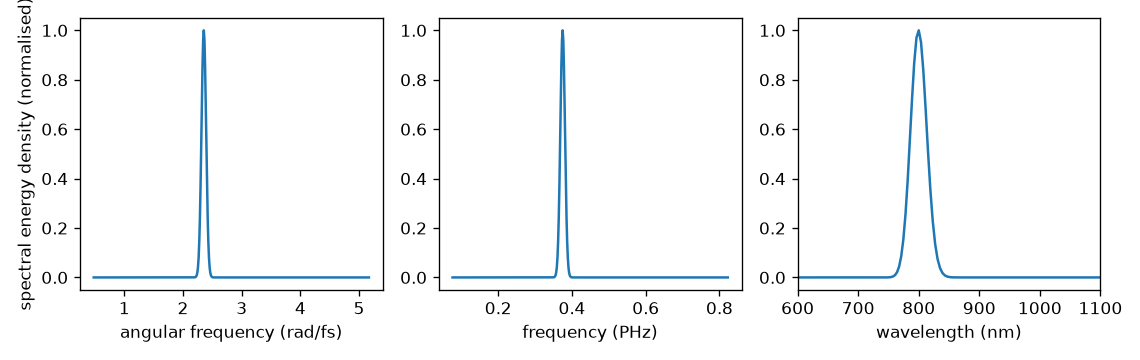
The same plane on the three abscissae. Each curve integrates to the pulse energy; the wavelength axis is returned ascending, which means the density has been reversed with it.#
The time domain, once#
There is one path from a stored spectrum to a time-domain quantity, and everything else is
a phasor away from it. On a field grid the real field is transformed back and
analytic_signal() applied; on an envelope grid the state already
is the analytic signal with its carrier removed. That pair is what
solprop.stats works with, and \(|\cdot|^2\) is the power in watts on both, so a
power read here is bit-identical to a power recorded during the run. The carrier is put
back only for the representation that wants it:
Oversampling zero-pads the spectrum, which is exact interpolation of a band-limited trace,
and returns the grid’s own fine time axis: centred on zero, of length
oversampling * n_t.
On that one path two things may be done to the spectrum before it is transformed, in this
order and after any band pass. transform_limit=True discards the spectral phase,
giving the shortest pulse the spectrum supports (the Fourier transform limit), centred
on \(t=0\).
transfer= applies a linear optical element of solprop.optics — a Taylor
phase, a thickness of glass, chirped-mirror reflections — so that
get_field() and get_power()
return the pulse as it arrives after a compressor. The elements,
and the searches that choose their parameters, are on
the compression page. With neither keyword the spectrum is
transformed untouched.
The spectral phase, without a ramp#
A raw DFT spectrum has its phase origin at the first time sample, so a pulse at the
centre of the window carries a linear ramp \(\omega T/2\) in its phase. The optics
convention of the stored spectrum has already moved that origin to the centre of the
window — the \((-1)^k\) of spectrum_to_optics() — so
get_phase() subtracts no ramp: a flat phase means a
transform-limited pulse at the centre of the window, and the curvature is the group-delay
dispersion with the textbook sign.
import matplotlib.pyplot as plt
import numpy as np
from solprop.processing import get_phase, grid_of
from solprop.processing._examples import example_output

output = example_output()
grid = grid_of(output)
beta2 = output.metadata.configuration["beta2"]

omega, first = get_phase(output, plane=0)
_, last = get_phase(output, plane=-1)
inband = np.abs(omega - grid.omega0) < 0.15 * grid.omega0
added = (last - first)[inband]
expected = 0.5 * beta2 * (omega[inband] - grid.omega0) ** 2 * grid.length

fig, ax = plt.subplots(figsize=(5.4, 3.2))
ax.plot((omega[inband] - grid.omega0) * 1e-15, added - added[added.size // 2],
        lw=3, alpha=0.4, label="measured")
ax.plot((omega[inband] - grid.omega0) * 1e-15,
        expected - expected[expected.size // 2], "k--", lw=1, label="beta2 z / 2")
ax.set_xlabel("omega - omega0 (rad/fs)")
ax.set_ylabel("added spectral phase (rad)")
ax.legend(frameon=False)
fig.tight_layout()
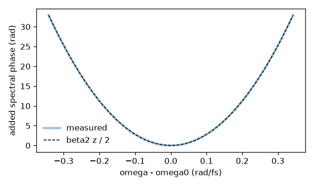
The spectral phase a known group-velocity dispersion adds over the length of the example run, against the parabola it should be. Positive dispersion is a positive parabola, as it is in the optics convention.#
The metrics#
solprop.processing.time measures the pulse. Where solprop.stats
already has the definition it calls it, so a number read off a saved run and the same
number recorded during the run agree to the bit; where it does not, the definition lives
here.
The two temporal powers. There is one exception to that bitwise agreement, and it is
a matter of what a file can know rather than of two implementations. A run evaluates its
temporal statistics from the internal amplitude and the plane’s index, as the analytic
Poynting flux \(P(t)=\sum_p\operatorname{Re}[a(t)a_w(t)^*]\) of
power and intensity. A saved plane holds only the true-power
amplitude \(b=\sqrt w\,a\) and no mode, so
peak_power() and
fwhm_t() — and
get_power(), the trace they are read off — measure
\(|b(t)|^2\) instead. The two kernels differ only in taking the geometric rather than the
arithmetic mean of \(w(\omega)\) and \(w(\omega')\), so the difference is second order in the
variation of \(\operatorname{Re}n_{\rm eff}\) across the spectrum: of order \(10^{-7}\) of
the peak for a gas-filled capillary (\(7.95\times10^{-8}\) measured on a shortened six-mode
hydrogen-filled capillary). Their time integrals agree exactly by Parseval, so
energy() is unaffected. Quote the run’s own value, in
stats/, where the distinction matters; divide a plane by \(\sqrt w\) from
solprop.processing.mixtures.get_power_weight() to reproduce the flux by hand.
metric |
units |
definition |
|---|---|---|
J |
|
|
W |
|
|
s |
|
|
Hz |
The width at half maximum of the density on the frequency axis. |
|
– |
\(\Delta t \, \Delta\nu\), which is \(2\ln 2/\pi = 0.4413\) for a transform-limited Gaussian. The mode selection applies to both widths. |
|
s |
The first moment of the power, or the time of its peak. |
|
J |
\(\int E_a^{*}(t) E_a(t+\tau)\,\mathrm{d}t\), whose value at zero delay is the pulse energy. |
|
W²s |
\(\int P(t) P(t+\tau)\,\mathrm{d}t\), what an autocorrelator measures. |
|
s |
The width at half maximum of \(|A(\tau)|^2\), with \(A\) the field autocorrelation above; \(2\sqrt{\ln 2}/\Delta\omega\) for a Gaussian spectrum of angular width \(\Delta\omega\). |
Three general helpers come with them:
fwhm() and
half_max_range(), which measure any trace with the two
conventions solprop.stats uses for the temporal power – through the same
crossing code, so a width measured here and the one recorded during the run are one
number – and
moment().
Modes are not summed unless you say so#
modes=None gives one number per mode, modes=2 gives that mode’s, and modes="sum"
gives the number of the total. What “the total” means depends on the quantity: for an
energy or a density the modes are added, for a peak power the powers are added before
the maximum is taken, and for a complex amplitude a modal sum is refused, because
modal amplitudes only add at a point in space and adding them anywhere else is a
convention nobody asked for. Polarisation components, by contrast, are always summed in a
quadratic quantity: they are two components of one field and their powers add at every
instant.
Smoothing to an instrument resolution#
specres() puts a density on a uniform axis and
convolves it with a unit-area Gaussian whose full width at half maximum is the stated
resolution, weighted by the width of the bin each value came from:
Because the kernel integrates to one, so does the result: the energy is preserved wherever the signal is well inside the range. The input axis need not be uniform, which is what makes this work directly on a wavelength axis derived from a uniform frequency grid — pass the bin widths, which the accessor does for you. Zero and negative values in the result are left as they are rather than replaced by a small positive number for the sake of a logarithmic plot, because that would change the data; clip them yourself when you plot.
import matplotlib.pyplot as plt
from solprop.processing import get_spectral_density
from solprop.processing._examples import example_output

output = example_output()
fig, ax = plt.subplots(figsize=(5.6, 3.2))
x, density = get_spectral_density(output, "wavelength", plane=-1)
ax.plot(x * 1e9, density, lw=1, label="unsmoothed")
for resolution in (20e-9, 60e-9):
    x, density = get_spectral_density(
        output, "wavelength", plane=-1, resolution=resolution
    )
    ax.plot(x * 1e9, density, label=f"{resolution * 1e9:.0f} nm")
ax.set_xlim(600, 1100)
ax.set_xlabel("wavelength (nm)")
ax.set_ylabel("spectral energy density (J/m)")
ax.legend(frameon=False)
fig.tight_layout()
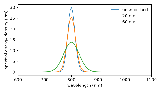
The same spectrum at three instrument resolutions. The area under each curve is the same; only the structure goes.#
Bandpass windows#
bandpass() builds a Planck taper that is one inside a
wavelength range and zero outside it, and returns it. The field accessors take it as
the bandpass keyword, either as the pair of wavelengths or as the array itself, which is
how a different edge from the default is asked for; bandpass(grid, limits, width=...)
sets the edge width in rad/s.
Each edge lies outside the pass band, and by default it is the narrower of 64
frequency bins (DEFAULT_BANDPASS_BINS, Luna’s
winwidth = :auto) and a quarter of the band’s angular width
(DEFAULT_BANDPASS_FRACTION). A Planck edge is
antisymmetric about its midpoint, so it transmits half its width, and a window with edges
\(f\) times the band’s width \(\Delta\omega\) has the integrated width
\((1 + f)\,\Delta\omega\). A fixed 64 bins is a fixed number of bins, not a fixed width: on
a 400 fs window it is several times wider than a 20 nm pass band, and the window would
transmit mostly its own edges. With \(f = 1/4\) the edges add at most a quarter of the band,
each still spans a quarter of it so the window stays smooth on the band’s own scale, and
every band wider than 256 bins keeps the 64-bin edge.
Coherence across an ensemble#
g12() is the first-order coherence of Dudley and
Coen: the modulus of the normalised cross-correlation of the spectra of independent noise
realisations, at each frequency,
evaluated with \(\sum_{i \neq j} \tilde E_i^{*} \tilde E_j = |\sum_i \tilde E_i|^2 - \sum_i |\tilde E_i|^2\), which is one pass over the ensemble rather than \(N^2\) slices. Identical realisations give exactly one; independent ones give zero in the mean. The diagonal \(i = j\) is excluded deliberately: keeping the self-terms in the numerator would give \(1/N\) rather than zero for a fully incoherent ensemble.
A worked example#
import numpy as np
from solprop.processing import (
    energy, fwhm_t, get_spectral_density, get_power, time_bandwidth,
)

wavelength, density = get_spectral_density(output, "wavelength", plane=-1)
t, power = get_power(output, plane=-1, oversampling=4)

print(f"{float(energy(output, plane=-1)) * 1e6:.3f} uJ")
print(f"{float(fwhm_t(output, plane=-1)) * 1e15:.1f} fs")
print(f"time-bandwidth product {float(time_bandwidth(output, plane=-1)):.3f}")
Reading a run from disk goes through a handler that is open: during the run it already
is, and afterwards open_file() opens the file read-only
through the same protocol, as a context manager if you like.
resume() returns the last plane only; it is for continuing a
run, not for reading one.
from solprop.output import open_file

with open_file("run.h5") as output:
    wavelength, density = get_spectral_density(output, "wavelength", plane=-1)