Hollow planar waveguides#
A hollow planar guide confines the field between two plates and leaves the other transverse direction open. Choose between a field uniform in that direction, whose energy is reported per unit width, and a resolved finite beam, whose energy is in joules. This choice determines whether transverse self-focusing or modulation instability can be represented.
SlabMode is the hollow planar (slab) guide of the
high-energy compressors: two parallel dielectric or metal plates at \(x=\pm a\) with a
gas-filled gap \(2a\), free in y (Akturk et al. 2009, 12.5 mJ to 13.6 fs; Arnold et al.
2010, 10.6 mJ at 10.1 fs). This section models the guide uniform in y: the field
is a plane wave in the free direction and every transverse integral is taken over x
per metre of y. Energy then scales with the beam’s width in y at a fixed
intensity, which is what makes the geometry attractive, and what the model below
reports per unit width (see Per unit width).
from solprop.modes import ModeCollection, SlabMode

mode = SlabMode(63.5e-6, "Ar", 1.0)  # TE1, E along y, silica plates
modes = ModeCollection.slab(63.5e-6, (1, 3, 5), "Ar", 1.0)
TE and TM. polarisation="te" (the default) has its electric field along y,
parallel to the plates; "tm" has it along x, normal to them. The cited compressors use
TE, because a wave polarised parallel to a glass wall reflects at grazing incidence
far better than one polarised in the plane of incidence: TM loses \(\epsilon_{\rm
cl}/\epsilon_{\rm co}\) times more, 2.1 times for silica, and about \(n^2+\kappa^2\)
times more against a metal (Miyagi et al. eq. 36): \(n^2+\kappa^2=31\) for silver
at 800 nm, where the full model gives 33.
The two are distinct modes with their own effective index, each a row of its own;
with_polarisations() pairs them.
The model. The slab is the rectangular guide with one wall pair, the limit \(b\to\infty\) of Laakmann and Steier’s eq. (5), which is also Miyagi, Hongo and Kawakami’s eq. (19) and Arnold et al.’s eqs. (2)–(3):
with \(s=\sqrt{\epsilon_{\rm cl}-\epsilon_{\rm co}}\), \(\epsilon_{\rm co}=1+\chi\) the filled core and \(p=1,2,\dots\) the order. The two coefficients, the filled-core contrast and the permittivity ratio are the rectangular guide’s, written once and shared; the complex wall term stays in \(\beta\) for the reason given there. The profile is \(\cos(p\pi x/2a)\) for odd \(p\) and \(\sin(p\pi x/2a)\) for even \(p\) inside the gap and zero outside. To first order the field attenuation is
so the loss grows as \(p^2\) and as \(a^{-3}\), and the model is valid while
\(p\lambda/4a\ll1\) and the grazing angle lies well past Brewster’s (Laakmann’s
conditions 1–2). As for the rectangular guide, a mode warns once
(GrazingIncidenceWarning) wherever \(p\lambda/4a\) or
\(\lambda|q|/2\pi a\) exceeds 0.1 over the evaluated band, the threshold and its
reason being the ones given there.
For Akturk’s guide (a = 63.5 µm, 800 nm, silica, TE) it is
0.149 m⁻¹: 5.8 % of the power is lost in 20 cm, and 41 % of the third order’s, as
they print. Arnold’s statement that \(p=3\) is damped nine times and \(p=2\) four times
more than \(p=1\) is the \(p^2\) law.
Against a capillary. Taking the half-gap equal to a capillary’s radius, the TE fundamental loses \(1/(8(u_{11}/2\pi)^2(\nu^2+1))=0.275\) times what the capillary’s HE₁₁ does, and the TM fundamental \(\nu^2\) times that, 0.578 (\(\nu=1.45\)): one wall pair instead of a whole wall, and TE sees only the gentle reflection. The figure compares them across gaps.
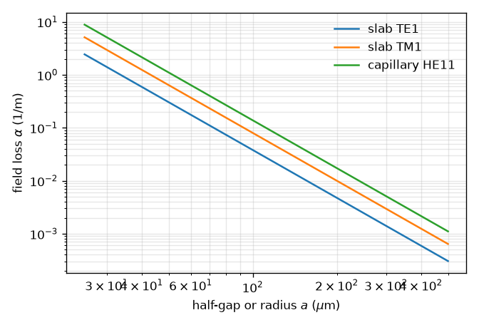
Field loss at 800 nm of the TE1 and TM1 modes of an evacuated silica slab against the half-gap a, beside the HE11 mode of a capillary of the same radius. All three fall as a^-3; TE1 is a quarter of the capillary and TM1 a little over half, the plates’ eps_cl/eps_co times TE1.#
Per unit width#
The normalisation and the effective “area” are integrals over x alone,
for every order: \(N\) is a power per metre of y for a unit amplitude, and
aeff() is an effective width in metres. It is
the protocol’s aeff and not a second name, so the mode-averaged normalisation and
\(\gamma'=n_2\omega/(cA_{\rm eff})\) read it unchanged. A run on slab modes therefore
reports power in W/m and energy in J/m from the same formulas; energy= and
peak_power= are per metre of y, and intensities (peak_intensity, fluence) are
still W/m² and J/m², being local. The mode declares
transverse_measure = "per_unit_width"
(TransverseMeasure), the run records it
(RunMetadata.transverse_measure, a key of the run configuration written only for
such a run), and
transverse_units() and the standard plots label
accordingly. A slab mode cannot share a set with an area mode: the collection
refuses it by name.
For a beam that is Gaussian in y, \(\exp(-(y/w_y)^2)\) in field with \(w_y\) the
1/e field radius (the 1/e² intensity radius), the total is
\(P=P'\,w_y\sqrt{\pi/2}\), and the same for energy:
per_unit_width_to_gaussian() and its inverse
gaussian_to_per_unit_width() convert. Akturk’s 12.5 mJ in
a beam of \(w_y=5\) mm is 2.0 J/m at its centre.
The rule, the launch and tapers#
The transverse rule of a slab set is Gauss–Legendre in x on \([-a,a]\), emitting
\((x,0)\) points with the weights \(a\,w_i\) times a unit y weight, so everything
downstream is the Cartesian pipeline with one y node. Its quartic products need the
same measured bound as a Cartesian axis: \(6h+6\) nodes
(cartesian_nodes()), re-measured on the
one-dimensional products (12, 17, 22, 26, 30 and 34 nodes reach \(10^{-12}\) for
\(h=1\) to 6). In prop_waveguide, n_r is the x node count and defaults
to the larger of the bound and the radial default; n_theta is refused. Unlike a
Cartesian product rule the slab rule takes the Kronrod extension (the default),
so the quadrature alarm runs and quadrature_error is recorded.
A beam focused into the gap is projected onto the modes by
gaussian_coupling(), the rule’s dual basis applied to
\(\exp(-(x/w_x)^2)\). A centred beam couples to odd orders only, so a multimode TE
set is (1, 3, 5); an offset one reaches the even orders. At \(w_x=0.735a\), 98.8 % of
the beam enters TE1, and 99.4 % of what falls inside the gap does (Arnold 2010,
§3.1). Two optima are worth telling apart: the share of the power
inside the gap that enters TE1 peaks at 0.735a (Arnold’s figure, and Laakmann’s
0.74a for the square guide), the share of the whole beam at 0.703a, where it is
98.9 % (Laakmann’s 0.69a). One linearly polarised beam launches one family: a set
with TE and TM rows needs component="y" (TE) or "x" (TM), and the other family
takes nothing. prop_waveguide places the pulse in the first mode; a projected
launch replaces that input with the pulse’s spectrum shared by these amplitudes,
through with_input():
import math

import numpy as np

from solprop.driver import Simulation
from solprop.modes import ModeCollection, gaussian_coupling
from solprop.pulses import GaussianPulse

modes = ModeCollection.slab(63.5e-6, (1, 3, 5), "Ar", 1.0)
simulation = Simulation.from_waveguide(
    modes.modes,
    0.1,
    "Ar",
    1.0,
    lambda0=800e-9,
    wavelength_limits=(650e-9, 1000e-9),
    trange=1.2e-12,
    fwhm=100e-15,
    energy=0.5,
    envelope=True,
    plasma=False,
    raman=False,
    n_save=2,
)
shares = gaussian_coupling(modes.modes, 0.735 * 63.5e-6)
pulse = GaussianPulse(wavelength=800e-9, fwhm=100e-15, energy=0.5).build(
    simulation.grid
)[0]
launch = np.stack([math.sqrt(share) * pulse for share in shares])
projected = simulation.with_input(launch)
A varying half-gap is a scale-invariant taper: the profile is a function of
\(x/a(z)\), the normalised field goes as \(a^{-1/2}\) and the weights as \(a\), so the
matrices rescale by \(\sqrt{a(0)/a(z)}\) (taper_scale())
and the mode-averaged area path works as for a capillary. The route omits the
connection \(\langle\psi_m|\partial_z\psi_n\rangle\) a taper drives between orders of
the same parity and says so (AdiabaticTaperWarning): each channel follows its local
mode adiabatically (S. Chen et al. 2011 model a tapered planar compressor; their δ is a
power attenuation). A gas fill between plates keeps the uniform flow law: the
fill ignores a varying gap.
What a slab uniform in y cannot show#
The energy limit of a real planar compressor is set in the free direction: whole-beam self-focusing, filamentation and the modulational instability of a wide beam in y (Arnold et al. 2009: stable to \(B=k_0I_0n_2L\approx15.5\), with the experiments near 8). A field that is uniform in y has no structure in y to focus, break up or modulate, so none of this appears in a slab run, however large its B integral; its critical power has no meaning here either, and none is quoted. The model is the right one for the guided dimension – modal loss, dispersion, SPM and intermodal exchange in x – at the centre of a beam wide enough that its y structure evolves slowly. Resolving y needs slab modes in x times a Fourier transform in y, the hybrid transform of the next section.
Resolving y#
The hybrid planar transform expands the field in the slab modes of one gap in x and a raw Fourier transform in y,
the expansion of Arnold et al. 2010 (eq. (9)). It is exact, non-paraxial, in y: each
column \((p, k_y)\) propagates with its own longitudinal wave number, the channel’s
complex wall term \(\kappa_p^2 =
k^2\epsilon_{\rm co}-\beta_p^2\) taken from the mode itself (so the loss policy and the
wall model are the uniform slab’s), the free-space evanescent model beyond cutoff and
the prefactor \(-i\omega^2/(2\epsilon_0c^2\operatorname{Re}k_z)\). At \(k_y = 0\) this is
the uniform slab exactly, so a field uniform in y reproduces a slab run started from the
same internal amplitude – to 2e-10 over ten steps, for the Kerr, Raman, field-plasma and
envelope-plasma responses and both absorber schemes. A planar run measures its slab
amplitudes with the explicit slab metric of
energy and flux in a medium: the weight of
column \((p, k_y)\) is \(c\operatorname{Re}q/\omega\) with
\(q=\sqrt{(\omega n_{{\rm eff},p}/c)^2-k_y^2}\), which at \(k_y = 0\) is \(\operatorname{Re}n_{\rm eff}\),
the weight of the true-power amplitude prop_waveguide launches
(power and intensity). A mode launched with the same
energy therefore has the same internal amplitude, \(|a|^2 = P/\operatorname{Re}n_{\rm eff}\),
on both routes. A Gaussian beam in y diffracts as the (1+1)-D Gaussian beam,
\(w(z)=w_0\sqrt{1+(z/z_R)^2}\) with axial amplitude \((1+(z/z_R)^2)^{-1/4}\) and Gouy phase
\(\tfrac12\arctan(z/z_R)\), times each mode’s own loss and dispersion (measured within
2e-6 of the paraxial forms, whose own error is \(O(1/(kw_0)^2)\)).
The grid is PlanarGrid: the slab channels (one gap, one
polarisation family, a constant gap and fill), the slab rule in x (the modal route’s
default node count) and a periodic y axis with the Cartesian grid’s collar. The state’s
columns are \((p, k_y)\) with the channel fastest; the geometry integrates over y, so a run
reports energy in J and power in W, not per unit width. The launch is a
PlanarPulse, a Gaussian of 1/e field radius \(w_x\) projected onto
the modes (with signs, gaussian_projection()) times a Gaussian
or super-Gaussian of radius \(w_y\) in y; its energy is the incident beam’s physical energy
in the fill, so the modes carry the coupled share of it.
from solprop.driver import Simulation, SimulationSettings
from solprop.grid import EnvelopeGrid
from solprop.modes import PlanarGrid, SlabMode
from solprop.pulses import GaussianPulse, PlanarPulse
from solprop.stepper import PIController

grid = EnvelopeGrid.from_limits(0.1, 800e-9, (650e-9, 1000e-9), 400e-15)
modes = [SlabMode(63.5e-6, "Ar", 1.0, order=p) for p in (1, 3)]
space = PlanarGrid(modes, 1e-3, 32)
launch = PlanarPulse(
    GaussianPulse(wavelength=800e-9, fwhm=100e-15, energy=1e-3),
    400e-6,
    waist_x=0.735 * 63.5e-6,
)
settings = SimulationSettings(
    controller=PIController(rtol=1e-6, atol=1e-9),
    save_planes=[0.1],
    dz_max=0.02,
    dz_init=0.02,
    backend="numpy_ref",
)
simulation = Simulation.from_planar(grid, space, [], launch, settings=settings)
print(simulation.translate().transform.geometry.kind, space.n_columns)
prop_planar(grid, space, responses, launch, settings=settings) builds the same
simulation and runs it in one call; the empty response sequence above is a linear
check, and a real run passes its Kerr, Raman and plasma responses there.
What it adds is everything in y: whole-beam self-focusing, and the modulational
instability of a wide beam that sets a planar compressor’s energy limit. The
constraints are the free-space grid’s: constant media (a gas path is refused) and here
also a constant gap, since a varying gap moves the slab modes under the frozen operator,
which the hybrid transform does not support; the state is scalar, so TE and TM are
not mixed. critical_power() accepts a planar grid and returns
the material quantity: Arnold et al. (2009, section 2.1) quote a planar compressor
against \(P_c = 2\pi n_0/(k_0^2 n_2)\), “the critical power for 2D collapse”, writing both
the whole-beam self-focusing length \(L_{\rm sf}\) and the modulational-instability length
\(L_{\rm mi}\) in terms of \(P/P_c\) of the power in the guide. The plates stop the whole
beam collapsing as it would in free space, but a multimode x basis can still focus in
x. Their \(P_c\) is \(2n_0^2/1.86226\) times the function’s value (called with index=n0),
the Gaussian mass against the Townes one and the \(n_0^2\) of their \(n_2\) convention. numpy_ref, numba_cpu and the native CPU backend execute the
transform: the y FFT around the slab rule’s synthesis and projection, each column’s
operator with its channel’s wall term, every response family, both absorber schemes and
the statistics, and both compiled backends agree with numpy_ref within derived
bounds. The hybrid planar transform has not been qualified on a GPU build of the native backend.
Planar compressors#
A planar compressor broadens a pulse by self-phase modulation in the TE1 mode. The beam’s width in y sets its energy at a fixed intensity, so the intensity can be held where argon barely ionises (a few \(10^{13}\) W/cm²) whatever the energy. What limits it is the beam’s behaviour in y, which the hybrid transform resolves.
Whole-beam self-focusing. Arnold et al. (2009, section 2.1) give its length for a frozen Gaussian profile as \(L_{\rm sf}=2\pi z_R\,(P^*/P_c)\,[4(P^*/P_c-1)]^{-3/2}\). Here \(z_R=k_0w_y^2/2\), \(P^*=\pi I_0w_y^2/2\), and \(P_c\) is their critical power above. For a beam several millimetres wide this is metres.
Modulational instability in y. Ripples on the beam grow at most as \(e^B\), where \(B=k_0n_2I_0L\). The distance at which the beam breaks up is therefore set by the B integral, and depends on the beam’s imperfections only through their logarithm. For their laser’s measured profile, Arnold et al. found stable propagation up to \(B\approx15.5\); their experiment ran near 8.
The planar compressor worked example runs their Table 1 experiment (a 127 µm gap between silica plates, 1.5 atm of argon, 21 cm, 8.7 mJ in 43 fs). It shows:
the modal shares at launch;
the transmission against Arnold’s closed-form loss;
the broadened spectrum, and the pulse at the beam centre compressed by a second-order phase;
the compressed duration and the fluence across y;
the B integral along the guide, and a beam seeded with weak noise in y that breaks up as B approaches Arnold’s limit.
A caveat in the literature#
Chen et al., OL 33, 2992 (2008), eq. (2), write the attenuation with \(\nu\), the cladding-to-core index ratio, where Laakmann’s TE coefficient is \(1/\sqrt{\nu^2-1}\): 52 % high for TE and 28 % low for TM at \(\nu=1.45\) (58 % and 27 % at Pyrex’s 1.47). It is not implemented; the numbers above are Laakmann’s, Miyagi’s and Arnold’s.
References: K. D. Laakmann and W. H. Steier, Applied Optics 15, 1334 (1976), doi:10.1364/AO.15.001334; M. Miyagi, A. Hongo and S. Kawakami, IEEE J. Quantum Electron. QE-19, 136 (1983), doi:10.1109/JQE.1983.1071837; C. L. Arnold et al., New J. Phys. 12, 073015 (2010), doi:10.1088/1367-2630/12/7/073015; C. L. Arnold et al., Opt. Express 17, 11122 (2009), doi:10.1364/OE.17.011122; S. Akturk et al., Opt. Lett. 34, 1462 (2009), doi:10.1364/OL.34.001462; J. Chen et al., Opt. Lett. 33, 2992 (2008), doi:10.1364/OL.33.002992; S. Chen et al., J. Opt. Soc. Am. B 28, 1009 (2011), doi:10.1364/JOSAB.28.001009.