Note
Go to the end to download the full example code.
A planar hollow-waveguide compressor#
In a hollow capillary the bore fixes the beam’s area. The energy it can compress is therefore bounded by the intensity at which the gas ionises or the entrance is damaged, and a larger bore raises the bound only at the cost of a longer guide. A planar hollow waveguide removes the bound in one direction. Two polished glass plates, a fraction of a millimetre apart, guide the beam in one direction only (x, across the gap). In the other direction (y, along the plates) the beam is free, so it can be made as wide as the energy needs to keep the intensity where self-phase modulation broadens the spectrum and the gas barely ionises. Akturk et al. (Opt. Lett. 34, 1462 (2009)) compressed 12.5 mJ pulses from 45 fs to 13.6 fs this way, with 8.1 mJ leaving the guide, and Arnold et al. (New J. Phys. 12, 073015 (2010)) reached 10.6 mJ at 10.1 fs.
The free direction is also where such a compressor fails. The Kerr effect that broadens the spectrum also focuses the beam in y. The whole beam self-focuses slowly, and small ripples on it grow by modulational instability (MI) until the beam breaks up into filaments. Arnold et al. (Opt. Express 17, 11122 (2009)) put the limit at a B integral \(B = k_0 n_2 I_0 L \approx 15.5\) for their laser’s measured beam profile, with the experiment near 8.
This example models the experiment of their Table 1 (the Akturk 2009 guide) with the hybrid planar transform (Hollow planar waveguides, “Resolving y”). The field in the gap is a sum of slab modes in x, each with an amplitude that depends on y and t. The modes carry the guide’s loss and dispersion. The y direction is a Fourier transform, and diffraction in y uses the represented angular-spectrum operator. The guide has a 127 um gap between fused-silica plates and is 21 cm long, filled with 1.5 atm of argon. The pulse is 8.7 mJ and 43 fs long at 800 nm, focused to a line 50.2 um high (x) and 7.2 mm wide (y). The example follows the pulse through the guide, compresses it, and then runs a slightly noisy beam through a longer guide to show the break-up that sets the limit.
What to look for.
The launch puts 98 % of the beam into the fundamental TE1 mode. The higher modes are damped as \(p^2\), so the transmission follows Arnold’s closed-form loss closely. Arnold’s model gave about 93 %; the experiment gave 65 %, for reasons the model leaves out (listed below).
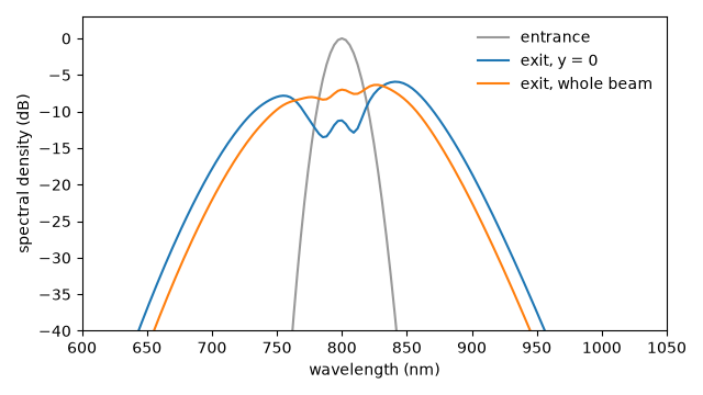
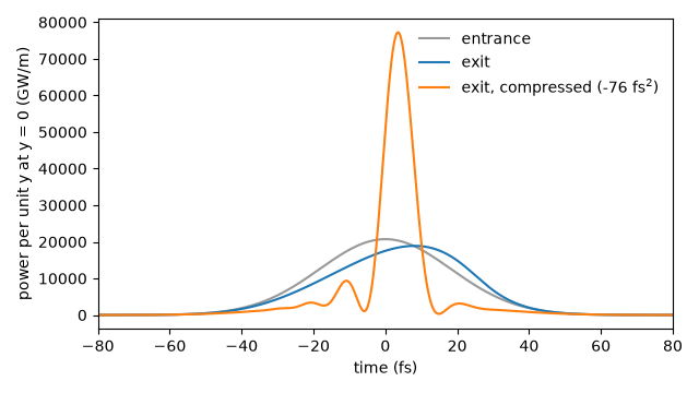
At the beam centre the spectrum broadens by self-phase modulation, and a second-order phase alone (about -76 fs²) compresses the pulse from 43 fs to about 9 fs, close to its transform limit (Akturk measured 13.6 fs, from a measured rather than ideal input pulse).
Across y the broadening follows the beam profile: the wings are compressed less. Arnold et al. (2010) found that 71 % of the energy lies where the compressed pulse is shorter than 1.5 times its duration at the centre (67.6 % measured). The example computes the same share.
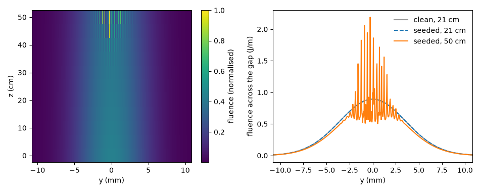
With a clean Gaussian beam the fluence across y stays smooth at the exit, where the B integral is about 8.7. With a seed of one part in \(10^5\) in the field across y, ripples grow at the centre of the beam, at about the MI period of a quarter of a millimetre. They grow roughly as \(e^{0.55B}\), not the \(e^B\) of the fastest-growing ripple in the linear theory: the fluence averages over the pulse and the beam’s wings, where the gain is lower, and white noise puts only a small part of its power near the fastest period. At the 21 cm exit they are a few parts in \(10^4\). By 40 cm, at B of about 17, the rms ripple is 4 %; beyond, the beam breaks up into filaments that self-focus, so the peak intensity, and with it the B integral, runs away (B of about 35 at 45 cm and 100 at 50 cm) and the ripple reaches 15 to 23 %. So at this seed the beam breaks up just beyond the limit Arnold place, \(B \approx 15.5\). (With solprop’s former argon Kerr coefficient, 23 % lower, B reached 16 only at 50 cm, where the beam was just beginning to break up.)
What is approximate.
The launch is an ideal Gaussian in x, y and time. Arnold’s simulation used the measured temporal pulse and beam profile, with the input energy corrected for the experiment’s extra loss; the 8.7 mJ used here is that corrected energy.
Four TE modes are kept: the odd orders 1, 3, 5 and 7, the only ones a centred beam excites. TE7 carries 0.1 % at launch and is damped fifty times more than TE1. Arnold used ten.
The Kerr effect is the only nonlinearity. Plasma is left out: optmat’s argon rate at the peak intensity leaves about 5e14 electrons per cubic centimetre (Arnold: “well below 1e15”), whose index change is about 3 % of the Kerr one (printed below). That estimate uses the incident peak intensity, so it does not justify the omission after strong spatial contraction: the late, under-resolved breakup is qualitative and cannot predict a filament peak intensity. Argon has no Raman response.
solprop’s nonlinear index for argon is optmat’s Kerr fit at the carrier (SEP 3), 5 % above the 0.98e-19 cm² W⁻¹ bar⁻¹ Arnold used (both printed below). The B integral here is the model’s own, so the same guide reaches a given B about 5 % sooner than in Arnold’s simulation.
The noise seed across y is a stand-in, not Arnold’s measured profile. Because MI grows exponentially, the B at which the beam breaks up depends on the seed only through its logarithm: ten times more noise lowers it by about ln 10 = 2.3.
The y window is ±18 mm, 2.5 times the beam radius, with 1024 samples. The samples resolve the linear MI band (wavenumbers up to 3.6e4 rad/m) with a margin of 2.2, but not the fine structure of the filaments after break-up.
The band runs from 450 nm to 1.6 um, inside the qualified ranges of optmat’s argon index (from 108 nm to the static limit) and Kerr fit (400 nm to 20 um); the range warnings of the grid’s padding beyond the band are silenced below.
The model leaves out what Arnold et al. give as the likely causes of the experiment’s lower transmission: inhomogeneities of the beam, imperfections of the guide, reflections at the cell windows and clipping of the beam inside the cell.
The set-up#
The numbers from Arnold et al. (2009), Table 1, first column. Before anything propagates, the closed forms give the regime:
the share of the launched beam each mode takes (the projection of the Gaussian onto the modes);
each mode’s loss, from Arnold’s eq. (3): the field decays at \(\alpha_p = (p\lambda/4a)^2 / (a\sqrt{n_g^2 - 1})\) with \(n_g = 1.45\);
the peak intensity \(I_0 = 2P/(\pi w_x w_y)\) of the incident beam;
the B integral over the guide;
the whole-beam self-focusing length of Arnold’s section 2.1.
import time
import warnings

import matplotlib.pyplot as plt
import numpy as np
from scipy.integrate import cumulative_trapezoid

from solprop import fourier
from solprop.backends.memory import estimate_memory
from solprop.constants import BAR, CHARGE_MASS_RATIO, EPS0, STD_ATMOSPHERE, C
from solprop.driver import Simulation, SimulationSettings
from solprop.exceptions import MaterialRangeWarning
from solprop.grid import EnvelopeGrid
from solprop.modes import PlanarGrid, SlabMode, gaussian_coupling
from solprop.nonlinear.envelope_plasma import linear_cycle_averages
from solprop.nonlinear.optmat_rates import OptmatRate
from solprop.nonlinear.responses import KerrResponse
from solprop.optics import stored_factor
from solprop.physdata import density, gamma3, n2
from solprop.processing.compression import compress_taylor
from solprop.processing.time import fwhm
from solprop.pulses import GaussianPulse, PlanarPulse
from solprop.spatial import SpatialFlux, SpatialMedium, planar_mode_energy
from solprop.stats import StatsSpec, default_spec
from solprop.stepper import PIController

HALF_GAP = 63.5e-6
"""Half the plate separation a, m (the gap is 127 um)."""

LENGTH = 0.21
"""Guide length, m."""

PRESSURE = 1.5 * STD_ATMOSPHERE / BAR
"""Argon pressure, bar (1.5 atm)."""

WAVELENGTH = 800e-9
"""Pump wavelength, m."""

ENERGY = 8.7e-3
"""Incident pulse energy, J."""

DURATION = 43e-15
"""Incident pulse duration (FWHM of the power), s."""

WAIST_X = 50.2e-6
"""1/e field radius of the line focus across the gap, m."""

WAIST_Y = 7.2e-3
"""1/e field radius of the beam along the plates, m."""

ORDERS = (1, 3, 5, 7)
"""The TE orders kept: the odd ones, which a centred beam excites."""

RADIUS_Y = 18e-3
"""Half-width of the y window, m, before its absorbing collar."""

N_Y = 1024
"""Samples across y."""

LONG = 0.5
"""Length of the guide the seeded beam is followed through, m."""

SEED = 1e-5
"""Root-mean-square relative field noise across y on the seeded beam."""

GLASS_INDEX = 1.45
"""The plates' index in Arnold's closed-form loss."""

ARNOLD_N2 = 0.98e-23 * PRESSURE
"""Arnold's nonlinear index of argon, m^2/W (0.98e-19 cm^2/W per bar)."""

started = time.perf_counter()
warnings.simplefilter("ignore", MaterialRangeWarning)

k0 = 2.0 * np.pi / WAVELENGTH
modes = [SlabMode(HALF_GAP, "Ar", PRESSURE, order=p) for p in ORDERS]
shares = gaussian_coupling(modes, WAIST_X)
alpha = (np.array(ORDERS) * WAVELENGTH / (4.0 * HALF_GAP)) ** 2 / (
    HALF_GAP * np.sqrt(GLASS_INDEX**2 - 1.0)
)
for order, share, loss in zip(ORDERS, shares, alpha, strict=True):
    print(
        f"TE{order}: {share:.2e} of the beam, field loss {loss:.3f} 1/m, "
        f"{np.exp(-2.0 * loss * LENGTH):.3f} of its power left after {LENGTH} m"
    )

peak_power = 2.0 * np.sqrt(np.log(2.0) / np.pi) * ENERGY / DURATION
intensity = 2.0 * peak_power / (np.pi * WAIST_X * WAIST_Y)
n2_argon = n2("Ar", pressure=PRESSURE, wavelength=WAVELENGTH)
print(
    f"incident peak power {peak_power * 1e-9:.0f} GW, peak intensity "
    f"{intensity * 1e-4:.3g} W/cm^2 (Arnold: 3.35e13)"
)
print(
    f"n2 {n2_argon:.3e} m^2/W here, {ARNOLD_N2:.3e} in Arnold's model; "
    f"B over {LENGTH} m: {k0 * n2_argon * intensity * LENGTH:.2f} here, "
    f"{k0 * ARNOLD_N2 * intensity * LENGTH:.2f} with Arnold's n2 (they quote 8)"
)

# Whole-beam self-focusing in y (Arnold 2009, section 2.1): the critical power for
# 2D collapse, the power of a round beam of the same intensity and radius, and the
# focusing length of a frozen Gaussian profile.
critical = 2.0 * np.pi / (k0**2 * n2_argon)
ratio = np.pi * intensity * WAIST_Y**2 / 2.0 / critical
rayleigh = k0 * WAIST_Y**2 / 2.0
focusing = 2.0 * np.pi * rayleigh * ratio * (4.0 * (ratio - 1.0)) ** -1.5
print(
    f"P*/Pc = {ratio:.0f}; whole-beam self-focusing length {focusing:.1f} m, "
    f"{focusing / LENGTH:.0f} guide lengths"
)

# The ionisation the model leaves out: optmat's argon rate, averaged over the optical
# cycle, over the incident Gaussian pulse at its peak intensity, and the index change of
# the electrons against the Kerr one. The average is the envelope plasma's own,
# (1/2 pi) int W(|a cos theta|) d theta, which ``linear_cycle_averages`` evaluates at
# every sample of the pulse from one vectorised call of the rate.
t = np.linspace(-4.0, 4.0, 4001) * DURATION
envelope = intensity * np.exp(-4.0 * np.log(2.0) * (t / DURATION) ** 2)
# The axial intensity is n0 eps0 c |E|^2 / 2 in the gas (SEP 34); the rate reads E.
n0 = float(np.real(SpatialMedium("Ar", pressure=PRESSURE).index(np.array([k0 * C]))[0]))
amplitude = np.sqrt(2.0 * envelope / (n0 * EPS0 * C))
rate = linear_cycle_averages(OptmatRate("Ar", WAVELENGTH), amplitude)
electrons = density("Ar", PRESSURE) * (1.0 - np.exp(-np.trapezoid(rate, t)))
omega0 = k0 * C
critical_density = EPS0 * omega0**2 / CHARGE_MASS_RATIO
print(
    f"electrons at the peak {electrons * 1e-6:.2g} cm^-3; their index change is "
    f"{electrons / (2.0 * critical_density) / (n2_argon * intensity):.1%} of the Kerr "
    "one"
)
TE1: 9.81e-01 of the beam, field loss 0.149 1/m, 0.939 of its power left after 0.21 m
TE3: 1.35e-04 of the beam, field loss 1.339 1/m, 0.570 of its power left after 0.21 m
TE5: 2.03e-03 of the beam, field loss 3.720 1/m, 0.210 of its power left after 0.21 m
TE7: 1.20e-03 of the beam, field loss 7.290 1/m, 0.047 of its power left after 0.21 m
incident peak power 190 GW, peak intensity 3.35e+13 W/cm^2 (Arnold: 3.35e13)
n2 1.567e-23 m^2/W here, 1.489e-23 in Arnold's model; B over 0.21 m: 8.65 here, 8.22 with Arnold's n2 (they quote 8)
P*/Pc = 4193; whole-beam self-focusing length 2.5 m, 12 guide lengths
electrons at the peak 3.5e+14 cm^-3; their index change is 1.9% of the Kerr one
The grid and the launch#
The time window is 400 fs, which the transform rounds up to 512 samples, 715 fs. The higher modes are slower: over 21 cm, TE3 falls 28 fs behind TE1 and TE7 170 fs, and both stay inside the window. (Over the 50 cm of the second run below, TE7 falls 400 fs behind and wraps around, but by then it carries less than 1e-6 of the energy.) The y window holds the beam out to 2.5 radii, where its intensity is 4e-6 of the peak, before the collar begins.
PlanarPulse projects the Gaussian line focus onto the
modes. Its energy is the incident beam’s, so what falls on the plates is lost at the
entrance, as in the experiment.
The statistics are recorded at every step as well as at the save planes: the energy for the transmission, and the peak intensity for the B integral.
def settings_for(planes):
    """Return the stepping and statistics of a run saving at `planes`."""
    return SimulationSettings(
        controller=PIController(rtol=1e-6, atol=1e-13),
        save_planes=planes,
        dz_max=5e-3,
        dz_init=1e-3,
        stats=StatsSpec(
            names=default_spec("free").names,
            periodic=("energy", "peak_intensity", "on_axis_intensity"),
        ),
    )


grid = EnvelopeGrid.from_limits(LENGTH, WAVELENGTH, (450e-9, 1.6e-6), 400e-15)
space = PlanarGrid(modes, RADIUS_Y, N_Y)
launch = PlanarPulse(
    GaussianPulse(wavelength=WAVELENGTH, fwhm=DURATION, energy=ENERGY),
    WAIST_Y,
    waist_x=WAIST_X,
)
kerr = [KerrResponse(gamma3("Ar", wavelength=WAVELENGTH), thg=False)]
print(space)

clean = Simulation.from_planar(
    grid, space, kerr, launch, settings=settings_for([LENGTH])
)

# The persistent memory of the run, before anything is allocated:
# ``estimate_memory`` gives 0.83 GB at this size, all of it the base group (the
# state, the stage buffers and the operator tables), for this run and for the seeded
# one below. The saved planes come on top, 34 MB each: two here, twelve there.
estimate = estimate_memory(clean.translate(), "auto")
print(f"estimated memory on {estimate.backend}: {estimate.total / 1e9:.2f} GB")
PlanarGrid: slab modes in x, periodic samples in y
  modes:           TE1, TE3, TE5, TE7
  gap:             127 um
  x nodes:         49 (slab rule)
  half-width in y: 18 mm, 1024 samples
  spacing in y:    38.67 um
  window factor:   0.1
  measure:         area: energy J, power W
estimated memory on native: 1.77 GB
The propagation#
Kerr only. The backend is the default, "auto", which is the native build where
one is installed.
clean_output = clean.run(progress="none")
print(clean_output)
print(
    f"peak intensity in the guide at the entrance "
    f"{clean_output['stats/peak_intensity'][0] * 1e-4:.3g} W/cm^2"
)


def rows_of(plane):
    """Return a saved plane as mode amplitudes at each y, shape (n_y, n_p, n_omega).

    The state's columns are the pairs (p, k_y), with p fastest; an inverse DFT over
    k_y gives the amplitudes on the y samples (``PlanarGrid``).
    """
    return np.fft.ifft(plane[:, 0].reshape(space.n_y, space.n_p, -1), axis=0)


def closure_of(plane, flux):
    """Return the magnetic closure of a saved plane as rows at each y.

    Each ``(p, k_y)`` column carries its own admittance ``c q / omega`` (SEP 34);
    the internal spectrum takes its conjugate.
    """
    return rows_of(np.conj(flux.admittance())[:, None, :] * plane)


flux = SpatialFlux.resolve(grid, space, clean.medium)
fields = clean_output.fields("fft")
entrance, exit_ = rows_of(fields[0]), rows_of(fields[-1])
entrance_g, exit_g = closure_of(fields[0], flux), closure_of(fields[-1], flux)
centre = int(np.argmin(np.abs(space.y)))
MemoryOutput
  state:           closed
  planes:          2, 0 m to 210 mm
  field per plane: 4096 x 1 x 512 (modes x components x omega)
  statistics:      beam_radius, energy, fwhm_r, on_axis_intensity, on_axis_spectrum, ...
  between planes:  energy, on_axis_intensity, peak_intensity
  run:             RunMetadata(slab, envelope grid of 512, 0 modes, native, 2026-10-2...
peak intensity in the guide at the entrance 3.25e+13 W/cm^2
Transmission#
The energy in the guide along z, as a share of the incident energy, against Arnold’s closed form: each mode keeps its launched share and loses power at \(2\alpha_p\), independently. The model departs from it where the Kerr effect moves energy between modes, and because loss grows as \(\lambda^2\) across the broadened spectrum.
z_steps = np.concatenate([[0.0], clean_output["step_stats/z"]])
energy = np.concatenate(
    [clean_output["stats/energy"][:1], clean_output["step_stats/energy"]]
)
closed = np.exp(-2.0 * np.outer(z_steps, alpha)) @ shares
fig, ax = plt.subplots(figsize=(6.4, 3.4))
ax.plot(z_steps * 100, energy / ENERGY, label="model")
ax.plot(z_steps * 100, closed, "--", label="Arnold's closed form")
ax.set_xlabel("z (cm)")
ax.set_ylabel("energy / incident energy")
ax.legend(frameon=False)
fig.tight_layout()
print(
    f"transmission {energy[-1] / ENERGY:.4f}; closed form {closed[-1]:.4f}; "
    "Arnold's model about 0.93, the experiment 0.65"
)
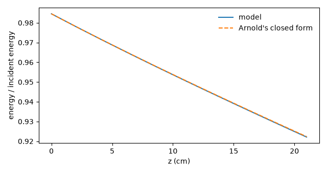
transmission 0.9221; closed form 0.9223; Arnold's model about 0.93, the experiment 0.65
Spectral broadening#
The spectrum at the beam centre, summed over the modes, and across the whole beam, each against the entrance on its own decibel scale. The centre, where the intensity is highest, broadens most; averaged over the beam, the wings add a narrower spectrum on top.
order = np.argsort(grid.omega)
wavelength = 2.0 * np.pi * C / grid.omega[order] * 1e9


def spectrum_db(rows, reference):
    """Return a spectrum summed over the modes, in dB below the reference's peak."""
    spectral = np.sum(np.abs(rows) ** 2, axis=tuple(range(rows.ndim - 1)))[order]
    peak = np.max(np.sum(np.abs(reference) ** 2, axis=tuple(range(rows.ndim - 1))))
    return 10.0 * np.log10(np.maximum(spectral / peak, 1e-12))


fig, ax = plt.subplots(figsize=(6.4, 3.6))
ax.plot(
    wavelength,
    spectrum_db(entrance[centre], entrance[centre]),
    color="0.6",
    label="entrance",
)
ax.plot(wavelength, spectrum_db(exit_[centre], entrance[centre]), label="exit, y = 0")
ax.plot(wavelength, spectrum_db(exit_, entrance), label="exit, whole beam")
ax.set_xlim(600.0, 1050.0)
ax.set_ylim(-40.0, 3.0)
ax.set_xlabel("wavelength (nm)")
ax.set_ylabel("spectral density (dB)")
ax.legend(frameon=False)
fig.tight_layout()
The compressed pulse#
Arnold et al. compressed their simulated pulse with a second-order phase alone,
standing in for chirped mirrors.
compress_taylor() searches that phase for
the highest peak power of the pulse at the beam centre, summed over the modes: the
power per metre of y there. It returns the phase, the durations and the transform
limit.
compression = compress_taylor(grid=grid, spectrum=exit_[centre][:, None, :], order=2)
print(compression)
gdd = compression.coefficients[2]
print(
    f"GDD {gdd * 1e30:.0f} fs^2 compresses the centre from "
    f"{compression.fwhm_before * 1e15:.1f} fs to "
    f"{compression.fwhm_after * 1e15:.1f} fs "
    f"(transform limit {compression.fwhm_limit * 1e15:.1f} fs; Akturk measured 13.6 fs "
    "with mirrors of about -300 fs^2)"
)

oversampling = 8
factor = stored_factor(grid, compression.transfer)
t_fine = (np.arange(oversampling * grid.n_t) - oversampling * grid.n_t / 2) * (
    grid.dt / oversampling
)


def power_in_time(rows, transfer=None):
    """Return the power per unit y summed over the modes, W/m, on the fine time axis."""
    stored = rows if transfer is None else rows * transfer
    fine = fourier.oversample(stored, oversampling * grid.n_t, kind=grid.kind)
    samples = fourier.inverse(fine, kind=grid.kind)
    return np.sum(np.abs(samples) ** 2, axis=-2)


fig, ax = plt.subplots(figsize=(6.4, 3.6))
ax.plot(
    t_fine * 1e15, power_in_time(entrance[centre]) * 1e-9, color="0.6", label="entrance"
)
ax.plot(t_fine * 1e15, power_in_time(exit_[centre]) * 1e-9, label="exit")
ax.plot(
    t_fine * 1e15,
    power_in_time(exit_[centre], factor) * 1e-9,
    label=f"exit, compressed ({gdd * 1e30:.0f} fs$^2$)",
)
ax.set_xlim(-80.0, 80.0)
ax.set_xlabel("time (fs)")
ax.set_ylabel("power per unit y at y = 0 (GW/m)")
ax.legend(frameon=False)
fig.tight_layout()
Compression by taylor
  found:      GDD -76.34 fs^2
  duration:   44.84 fs before, 9.185 fs after, 8.577 fs at the transform limit
  peak power: 18.89 TW before, 77.23 TW after, 90.72 TW at the limit
  quality:    0.8514 of the transform-limited peak power
  search:     converged: Solution found. (78 evaluations)
GDD -76 fs^2 compresses the centre from 44.8 fs to 9.2 fs (transform limit 8.6 fs; Akturk measured 13.6 fs with mirrors of about -300 fs^2)
Across the beam#
What happens in y, and where filamentation or MI would appear:
the fluence integrated across the gap at the entrance and at the exit;
the peak intensity on the mid-plane, x = 0, at each y;
the duration at each y after the phase that compressed the centre.
A clean Gaussian stays smooth: at B of about 8.7, numerical round-off is far too small a seed for MI to grow from, and whole-beam focusing needs metres. The wings see less self-phase modulation, so the centre’s phase compresses them less. The share of the energy within 1.5 times the centre’s duration is the number Arnold et al. (2010) give as 71 % (67.6 % measured).
def fluence_across(rows, closure):
    """Return the axial flux integrated over time and across the gap at each y, J/m.

    The slab modes are orthonormal in x, so the gap integral pairs each mode with
    its own closure.
    """
    weights = fourier.energy_weights(grid.n_omega, grid.dt, kind=grid.kind)
    return np.sum(weights * np.real(rows * np.conj(closure)), axis=(-2, -1))


def mid_plane_peak(rows, closure):
    """Return the peak axial intensity over time on the mid-plane at each y, W/m^2."""
    field = fourier.inverse(np.einsum("p,ypw->yw", space.centre, rows), kind=grid.kind)
    magnetic = fourier.inverse(
        np.einsum("p,ypw->yw", space.centre, closure), kind=grid.kind
    )
    return 0.5 * EPS0 * C * np.max(np.real(field * np.conj(magnetic)), axis=-1)


fluence = fluence_across(exit_, exit_g)
lit = fluence > 1e-3 * fluence.max()
durations = np.full(space.n_y, np.nan)
for index in np.flatnonzero(lit):
    durations[index] = fwhm(t_fine, power_in_time(exit_[index], factor))
within = lit & (durations < 1.5 * durations[centre])
print(
    f"{np.sum(fluence[within]) / np.sum(fluence):.1%} of the exit energy lies where "
    f"the compressed pulse is shorter than 1.5 x {durations[centre] * 1e15:.1f} fs"
)

fig, (top, middle, bottom) = plt.subplots(3, 1, figsize=(6.4, 7.2), sharex=True)
y_mm = space.y * 1e3
top.plot(y_mm, fluence_across(entrance, entrance_g), color="0.6", label="entrance")
top.plot(y_mm, fluence, label="exit")
top.set_ylabel("fluence across\nthe gap (J/m)")
top.legend(frameon=False)
middle.plot(y_mm, mid_plane_peak(entrance, entrance_g) * 1e-4, color="0.6")
middle.plot(y_mm, mid_plane_peak(exit_, exit_g) * 1e-4)
middle.set_ylabel("peak intensity\nat x = 0 (W/cm$^2$)")
bottom.plot(y_mm[lit], durations[lit] * 1e15)
bottom.axhline(1.5 * durations[centre] * 1e15, color="0.6", linestyle=":")
bottom.set_ylabel("compressed\nFWHM (fs)")
bottom.set_xlabel("y (mm)")
bottom.set_xlim(-2.5 * WAIST_Y * 1e3, 2.5 * WAIST_Y * 1e3)
fig.tight_layout()
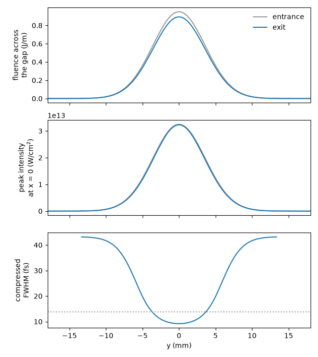
69.1% of the exit energy lies where the compressed pulse is shorter than 1.5 x 9.2 fs
A beam that is not clean#
A real beam carries small ripples across y. Here the launch is multiplied by
\(1 + \epsilon\,\xi(y)\), where \(\xi\) is white Gaussian noise of unit rms
on the y samples and \(\epsilon = 10^{-5}\). The noisy beam is then followed
through a guide of the same kind, 50 cm long, beyond the B integral of about 15.5
where Arnold place the limit. The launch is an internal (p, k_y) spectrum. It
is taken to y, where the noise multiplies it, and transformed back.
In the linear theory of MI in the (1+1)-D nonlinear Schroedinger equation, a ripple of wavenumber \(K\) grows as \(\exp(gz)\), with \(g = (K/2k)\sqrt{4kk_0n_2I - K^2}\). The fastest growth is \(k_0n_2I\) per metre, a factor \(e^B\) over the guide. Ripples grow for \(K\) up to \(2k_0\sqrt{n_2I}\), 3.6e4 rad/m here, and fastest at a period of 0.25 mm.
rng = np.random.default_rng(49)
noise = 1.0 + SEED * rng.standard_normal(space.n_y)
seeded_rows = (
    rows_of(launch.build(grid, space, medium=clean.medium)) * noise[:, None, None]
)
seeded_launch = np.fft.fft(seeded_rows, axis=0).reshape(space.n_columns, 1, -1)
planes = np.union1d(np.arange(1, 11) * LONG / 10, [LENGTH])
long_grid = EnvelopeGrid.from_limits(LONG, WAVELENGTH, (450e-9, 1.6e-6), 400e-15)
seeded = Simulation.from_planar(
    long_grid, space, kerr, seeded_launch, settings=settings_for(planes)
)
seeded_output = seeded.run(progress="none")
seeded_fields = seeded_output.fields("fft")
seeded_z = np.asarray(seeded_output["z"])
long_flux = SpatialFlux.resolve(long_grid, space, clean.medium)
seeded_fluence = np.array(
    [
        fluence_across(rows_of(plane), closure_of(plane, long_flux))
        for plane in seeded_fields
    ]
)
del seeded_fields
The B integral of both runs along z: the model’s own nonlinear phase at its peak, \(k_0 n_2 \int I_{\rm peak}\,dz\), with \(I_{\rm peak}\) the largest intensity anywhere in the beam at each step. The ripples are measured as the rms relative departure of the fluence from its own smooth part (wavenumbers below 5e3 rad/m, periods above 1.3 mm) within one beam radius of the centre.
def b_integral(output):
    """Return z and the cumulative B integral of a run at every step."""
    z = np.concatenate([[0.0], output["step_stats/z"]])
    peak = np.concatenate(
        [output["stats/peak_intensity"][:1], output["step_stats/peak_intensity"]]
    )
    return z, k0 * n2_argon * cumulative_trapezoid(peak, z, initial=0)


smooth_band = np.abs(space.k_y) < 5e3
inside = np.abs(space.y) < WAIST_Y


def ripple(profile):
    """Return the rms relative departure of a fluence profile from its smooth part."""
    smooth = np.real(np.fft.ifft(np.fft.fft(profile) * smooth_band))
    return float(np.sqrt(np.mean((profile[inside] / smooth[inside] - 1.0) ** 2)))


clean_z, clean_b = b_integral(clean_output)
long_z, long_b = b_integral(seeded_output)
plane_b = np.interp(seeded_z, long_z, long_b)
depth = np.array([ripple(profile) for profile in seeded_fluence])
for z, b, value in zip(seeded_z, plane_b, depth, strict=True):
    print(f"z = {z * 100:4.1f} cm: B = {b:5.2f}, fluence ripple {value:.2e}")
print(f"clean beam: B = {clean_b[-1]:.2f} at the exit, ripple {ripple(fluence):.1e}")
grown = np.flatnonzero(depth > 0.1)
if grown.size:
    print(f"the ripple first exceeds 10 % at B = {plane_b[grown[0]]:.1f}")
else:
    print(f"the ripple stays below 10 % up to B = {plane_b[-1]:.1f}")

fig, (left, right) = plt.subplots(1, 2, figsize=(9.5, 3.6))
left.plot(clean_z * 100, clean_b, label="clean, 21 cm")
left.plot(long_z * 100, long_b, "--", label="seeded, 50 cm")
left.axhline(15.5, color="0.4", linestyle=":")
left.axvline(LENGTH * 100, color="0.8")
left.text(1.0, 15.9, "Arnold's limit, 15.5", fontsize="small")
left.set_xlabel("z (cm)")
left.set_ylabel("B integral (rad)")
left.legend(frameon=False, loc="lower right")
right.semilogy(plane_b, depth, "o-", label="seeded beam")
guide = depth[1] * np.exp(plane_b - plane_b[1])
right.semilogy(plane_b, guide, ":", color="0.5", label="$e^B$, the fastest growth")
right.axvline(15.5, color="0.4", linestyle=":")
right.set_ylim(depth.min() / 3.0, 3.0)
right.set_xlabel("B integral (rad)")
right.set_ylabel("rms fluence ripple")
right.legend(frameon=False)
fig.tight_layout()
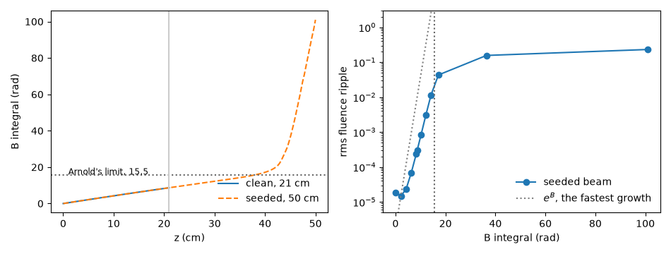
z =  0.0 cm: B =  0.00, fluence ripple 1.89e-05
z =  5.0 cm: B =  2.14, fluence ripple 1.47e-05
z = 10.0 cm: B =  4.24, fluence ripple 2.33e-05
z = 15.0 cm: B =  6.28, fluence ripple 6.76e-05
z = 20.0 cm: B =  8.29, fluence ripple 2.35e-04
z = 21.0 cm: B =  8.68, fluence ripple 3.03e-04
z = 25.0 cm: B = 10.24, fluence ripple 8.51e-04
z = 30.0 cm: B = 12.18, fluence ripple 3.13e-03
z = 35.0 cm: B = 14.22, fluence ripple 1.15e-02
z = 40.0 cm: B = 17.16, fluence ripple 4.31e-02
z = 45.0 cm: B = 36.42, fluence ripple 1.56e-01
z = 50.0 cm: B = 100.99, fluence ripple 2.31e-01
clean beam: B = 8.68 at the exit, ripple 1.7e-09
the ripple first exceeds 10 % at B = 36.4
The seeded beam’s fluence across y at every saved plane, and at the guide’s own length and at 50 cm, beside the clean beam at 21 cm. The gain is largest where the intensity is, so the ripples should appear first at the centre of the beam, at about the MI period, and spread outwards as they deepen into filaments.
fig, (left, right) = plt.subplots(1, 2, figsize=(9.5, 3.8))
image = left.pcolormesh(
    y_mm, seeded_z * 100, seeded_fluence / seeded_fluence.max(), shading="nearest"
)
left.set_xlim(-1.5 * WAIST_Y * 1e3, 1.5 * WAIST_Y * 1e3)
left.set_xlabel("y (mm)")
left.set_ylabel("z (cm)")
fig.colorbar(image, ax=left, label="fluence (normalised)")
at_length = int(np.argmin(np.abs(seeded_z - LENGTH)))
right.plot(y_mm, fluence, color="0.6", label="clean, 21 cm")
right.plot(y_mm, seeded_fluence[at_length], "--", label="seeded, 21 cm")
right.plot(y_mm, seeded_fluence[-1], label="seeded, 50 cm")
right.set_xlim(-1.5 * WAIST_Y * 1e3, 1.5 * WAIST_Y * 1e3)
right.set_xlabel("y (mm)")
right.set_ylabel("fluence across the gap (J/m)")
right.legend(frameon=False)
fig.tight_layout()
Runtime and reproducibility#
Two runs of four slab modes by 1024 samples in y by 512 in time: 21 cm with a clean beam and 50 cm with a seeded one.
backend = clean_output.metadata.backend
settings = backend.settings
print(
    f"{time.perf_counter() - started:.0f} s; backend {backend.name}, "
    f"{settings.get('thread_count', 'default')} threads"
)
567 s; backend native, 18 threads