Fewer source calls: the two integrators#

When the nonlinear response is expensive – a time-dependent Schrödinger equation at every radial node, say – response evaluations can dominate the run time. The default integrator, Multistep(), evaluates it once a step, reusing the sources of earlier steps (The Adams integrator); RungeKutta(), the interaction-picture DOPRI5 march, evaluates it seven times a step on the reference backend (Choosing a stepper).

This tutorial runs SEP 13’s canonical case, a 6 fs, 1 mJ pulse self-compressing in 4.2 m of helium with a gas-flow fill, both ways at the same tolerance, and counts the source calls from the step histories. The built-in Kerr and plasma responses are cheap, so here the two runs take seconds either way; with an expensive response the call count is a useful cost indicator, alongside measured time and achieved accuracy.

Two runs of the same fibre. The Adams run takes the default integrator: one call a step, its order chosen between one and five as it goes. The temporal collar is applied once per step (absorber_scheme="split_step"): the in-stage collar is a fast damping rate that would cap a multistep method’s step, and this pulse never reaches the collar, where the per-step split’s error would lie (the manual page explains both).

import matplotlib.pyplot as plt
import numpy as np

from solprop.driver import prop_capillary
from solprop.gasflow import steady_fill
from solprop.processing import fields
from solprop.stepper import RungeKutta

fill = steady_fill("He", [0.0, 2.1, 4.2], [0.0, 0.2, 0.0], radius=256e-6)
common = {
    "lambda0": 800e-9,
    "fwhm": 6e-15,
    "energy": 1e-3,
    "trange": 60e-15,
    "wavelength_limits": (90e-9, 1.6e-6),
    "rtol": 1e-3,
    "n_save": 50,
    "backend": "numpy_ref",
}
runge_kutta = prop_capillary(256e-6, 4.2, "He", fill, integrator=RungeKutta(), **common)
adams = prop_capillary(256e-6, 4.2, "He", fill, absorber_scheme="split_step", **common)

The source calls. Every attempted DOPRI5 step, accepted or rejected, costs seven evaluations on numpy_ref; every attempted Adams step costs one, plus one to start the history at the entrance and again on the far side of the gas-fill port at 2.1 m, where the run restarts its history across the kink in the density.

def attempts(output):
    """Return the number of attempted steps of a run."""
    return sum(plane.step_history.n_steps for plane in output.planes())


rk_calls = 7 * attempts(runge_kutta)
adams_calls = attempts(adams) + 2
print(f"IP-DOPRI5: {attempts(runge_kutta)} steps, {rk_calls} source calls")
print(f"Adams:     {attempts(adams)} steps, {adams_calls} source calls")
print(f"ratio:     {rk_calls / adams_calls:.1f}")

IP-DOPRI5: 109 steps, 763 source calls
Adams:     316 steps, 318 source calls
ratio:     2.4

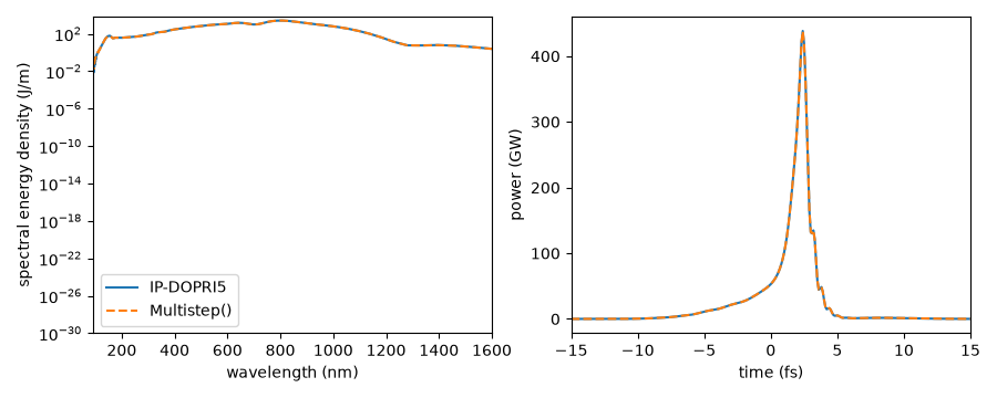
The same physics. The exit spectra agree over the whole band, including the weak ultraviolet below 200 nm, and the compressed pulses agree in time; the difference in the field is about 2e-3 of its norm here, a comparison at rtol=1e-3, not a bound on the global error of either run.

fig, (left, right) = plt.subplots(1, 2, figsize=(9.0, 3.6))
for output, label, style in (
    (runge_kutta, "IP-DOPRI5", "-"),
    (adams, "Multistep()", "--"),
):
    wavelength, density = fields.get_spectral_density(output, plane=-1)
    left.semilogy(wavelength * 1e9, density, style, label=label)
    time, power = fields.get_power(output, plane=-1)
    right.plot(time * 1e15, power / 1e9, style, label=label)
left.set_xlim(90, 1600)
left.set_ylim(1e-30, None)
left.set_xlabel("wavelength (nm)")
left.set_ylabel("spectral energy density (J/m)")
left.legend()
right.set_xlim(-15, 15)
right.set_xlabel("time (fs)")
right.set_ylabel("power (GW)")
fig.tight_layout()

reference = runge_kutta.fields()[-1]
difference = np.linalg.norm(adams.fields()[-1] - reference) / np.linalg.norm(reference)
print(f"exit field difference: {difference:.1e}")

exit field difference: 1.8e-03

Fewer source calls: the two integrators#

Related reading#