A pulse on both grids#

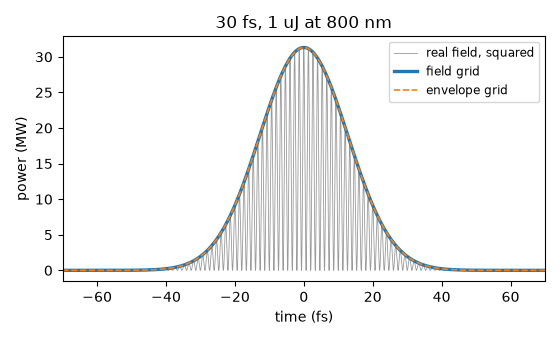
The same 30 fs, 1 uJ pulse at 800 nm, built on a field grid and on an envelope grid. The two representations store different things – a real electric field and a complex envelope about a carrier – but they describe one pulse, and solprop’s energy functional normalises both launches to the declared energy. Agreement of sampled curves still depends on bandwidth and temporal resolution.

Build the two grids over the same wavelength limits and time window, and the one pulse specification that will be built against both.

import matplotlib.pyplot as plt
import numpy as np

from solprop import fourier
from solprop.constants import C
from solprop.grid import EnvelopeGrid, FieldGrid
from solprop.noise import input_noise, photons_per_bin
from solprop.pulses import GaussianPulse

LIMITS = (400e-9, 2e-6)
TRANGE = 2e-12

field = FieldGrid.from_limits(1.0, 800e-9, LIMITS, TRANGE)
envelope = EnvelopeGrid.from_limits(1.0, 800e-9, LIMITS, TRANGE)

pulse = GaussianPulse(wavelength=800e-9, fwhm=30e-15, energy=1e-6)
spectra = {"field": pulse.build(field)[0, 0], "envelope": pulse.build(envelope)[0, 0]}

for name, grid in (("field", field), ("envelope", envelope)):
    energy = fourier.energy_omega(spectra[name], grid.dt, kind=grid.kind)
    print(f"{name:>9} grid: n_t = {grid.n_t:5d}, energy = {float(energy) * 1e6:.9f} uJ")

   field grid: n_t =  8192, energy = 1.000000000 uJ
envelope grid: n_t =  2048, energy = 1.000000000 uJ

In time, the field grid resolves every optical cycle and the envelope grid does not. The power is the modulus squared of the analytic signal on either grid, so the two curves lie on top of one another. The grey trace is the real field squared: its crests touch the envelope and its troughs reach zero twice in every optical cycle.

The default ffac = 6 sets fine-grid sampling from six times the highest retained frequency, enough for the band-limited field but too few to draw it smoothly. The spectrum is therefore zero-padded eight times over (solprop.fourier.oversample()) before the transform, which interpolates the represented periodic, band-limited field; it cannot recover frequencies absent from the original calculation.

fig, ax = plt.subplots(figsize=(5.6, 3.4))

OVERSAMPLING = 8
n_fine = OVERSAMPLING * field.n_t
fine = fourier.oversample(spectra["field"], n_fine, kind="field")
t_fine = (np.arange(n_fine) - n_fine / 2) * (field.dt / OVERSAMPLING)
carrier = fourier.inverse(fine, kind="field")
ax.plot(
    t_fine * 1e15,
    carrier**2 / 1e6,
    lw=0.6,
    color="0.6",
    label="real field, squared",
)
for name, grid in (("field", field), ("envelope", envelope)):
    samples = fourier.inverse(spectra[name], kind=grid.kind)
    if name == "envelope":
        signal = samples
    else:
        signal = fourier.analytic_signal(np.real(samples))
    style = {"lw": 2.4} if name == "field" else {"lw": 1.2, "ls": "--"}
    ax.plot(grid.t * 1e15, np.abs(signal) ** 2 / 1e6, label=f"{name} grid", **style)

ax.set_xlim(-70, 70)
ax.set_xlabel("time (fs)")
ax.set_ylabel("power (MW)")
ax.set_title("30 fs, 1 uJ at 800 nm")
ax.legend(fontsize="small")
fig.tight_layout()

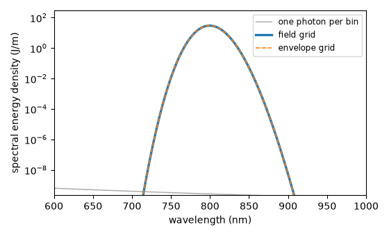
In frequency, the two grids sample different bins – the field grid is one-sided and the envelope grid is centred on its carrier – but the spectral energy density is one physical function of wavelength, so both trace the same curve. The shot-noise floor of one photon per bin is drawn underneath, on the envelope grid.

realisation = input_noise(envelope, np.random.default_rng(20260905))

fig, ax = plt.subplots(figsize=(5.6, 3.4))


def per_wavelength(spectrum, grid):
    """Spectral energy density per unit wavelength, sorted by wavelength."""
    density = fourier.spectral_density(spectrum, grid.dt, kind=grid.kind)
    band = grid.inband_mask
    wavelength = 2 * np.pi * C / grid.omega[band]
    order = np.argsort(wavelength)
    # dU/dlambda = dU/domega * 2 pi c / lambda^2.
    return wavelength[order], (density[band] * 2 * np.pi * C / wavelength**2)[order]


noise_wavelength, noise_density = per_wavelength(realisation.spectrum[0, 0], envelope)
ax.plot(
    noise_wavelength * 1e9,
    noise_density,
    lw=1.0,
    color="0.65",
    label="one photon per bin",
)
peak = 0.0
for name, grid in (("field", field), ("envelope", envelope)):
    wavelength, density = per_wavelength(spectra[name], grid)
    style = {"lw": 2.4} if name == "field" else {"lw": 1.2, "ls": "--"}
    ax.plot(wavelength * 1e9, density, label=f"{name} grid", **style)
    peak = max(peak, float(np.max(density)))

ax.set_yscale("log")
# The full dynamic range of the problem: the pulse peak at the top, the one-photon floor
# just above the bottom, and the Gaussian's flanks crossing it inside the plotted band.
ax.set_ylim(0.1 * float(np.max(noise_density)), 10.0 * peak)
ax.set_xlim(600, 1000)
ax.set_xlabel("wavelength (nm)")
ax.set_ylabel("spectral energy density (J/m)")
ax.legend(fontsize="small")
fig.tight_layout()

The photon number per bin says how far above the chosen one-photon noise floor the pulse sits, and it is exactly one in every active bin of the noise realisation – which is the definition the noise amplitudes come from (Conventions, section 4).

photons = photons_per_bin(envelope, spectra["envelope"])
floor = photons_per_bin(envelope, realisation.spectrum)[0, 0][envelope.active_mask]
print(f"peak photons per bin in the pulse: {float(np.max(photons)):.3e}")
print(f"photons per bin in the noise:      {float(np.mean(floor)):.12f}")

peak photons per bin in the pulse: 1.130e+11
photons per bin in the noise:      1.000000000000

A pulse on both grids#

Related reading#