Use tabulated hollow and solid-core modes

These rows are one converged JCMsuite finite-element solution of one fibre: 15 um core radius, 180 nm walls, six tubes of 10.38 um outer radius. The CSVs are exact copies of the vacuum and 10 bar argon rows of the reference data set solprop’s tests use (tests/data/jcmwave_vincetti.json), originally read from pyJCMwave’s library. Their headers identify the entries and source hash. They are not a universal accuracy reference. The gas comparison uses Kingston argon at 293 K. For a downloaded script, place the vacuum CSV and argon CSV in a data directory beside it.

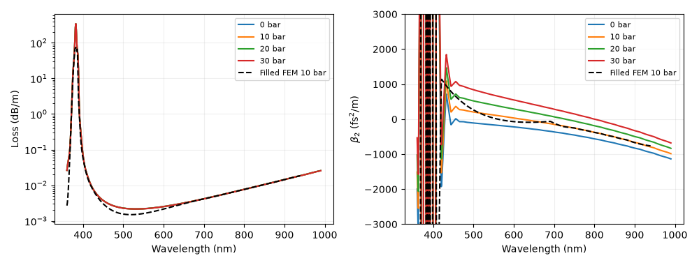
The vacuum table supports 200-1500 nm; the filled table supports 355-946 nm. Logarithmic imaginary-index interpolation preserves positive loss. The fixed-transverse-wavenumber rule predicts the nine smooth filled rows to 2.25e-8 in real index, but its near-resonance error reaches 2.83e-5. The filled table carries that one fill’s whole dispersion and loss. Its nonlinear material declaration must describe the same fill.

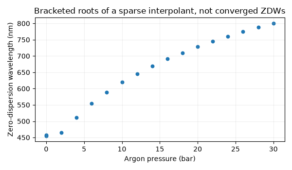
The ZDW plot shows roots bracketed by a 200-point scan on 450-990 nm, including two nearby roots of the sparse vacuum interpolant near 455-458 nm. Their physical interpretation needs refined data. This is a useful reason to inspect derivatives and leave-one-out error before interpreting a table as a physical prediction. No branch is silently discarded.

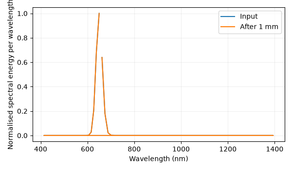
A reduced hollow example propagates a 10 nJ, 20 fs pulse at 650 nm for 1 mm in 1 bar argon. Its active band, including collars, lies inside the vacuum table. It uses eight radial nodes, Kerr only and 64 fixed steps: an interface example, not a converged broadband prediction. Finally a synthetic 200-knot solid-core table sampled from Taylor dispersion demonstrates the GNLSE n2 route, with unit prefactor index and no gas-material response inferred from the fibre.

import sys
from pathlib import Path
from time import perf_counter

import matplotlib.pyplot as plt
import numpy as np

from solprop.constants import C
from solprop.driver import Simulation, prop_gnlse
from solprop.grid import EnvelopeGrid
from solprop.log import NullReporter
from solprop.modes import IndexTable, TabulatedHollowMode, TabulatedMode
from solprop.modes.base import beta2, db_per_m, zdw
from solprop.nonlinear.gnlse import SpecifiedMode, attenuation_from_db
from solprop.stats import StatsSpec
from solprop.stepper import FixedSchedule

started = perf_counter()
# Gallery sets argv[0] to the source script but deliberately omits __file__. The
# tables are in a ``data`` directory beside the script.
data_directory = Path(sys.argv[0]).resolve().parent / "data"
vacuum = np.loadtxt(data_directory / "fem-vacuum.csv", delimiter=",")
argon = np.loadtxt(data_directory / "fem-argon.csv", delimiter=",")
table = IndexTable.from_wavelength(
    vacuum[:, 0], vacuum[:, 3] + 1j * vacuum[:, 4], area=vacuum[:, 6]
)
filled_table = IndexTable.from_wavelength(
    argon[:, 0], argon[:, 3] + 1j * argon[:, 4], area=argon[:, 6]
)
filled = TabulatedMode(
    15e-6,
    "Ar",
    10.0,
    temperature=293.0,
    table=filled_table,
    reference_wavelength=650e-9,
)

Keep derivative probes inside both tables. The filled overlay stops at 940 nm, before its last 946 nm row, and begins after its first row.

wavelength = np.linspace(360e-9, 990e-9, 600)
omega = 2 * np.pi * C / wavelength
figure, axes = plt.subplots(1, 2, figsize=(10, 3.8))
for pressure in (0.0, 10.0, 20.0, 30.0):
    mode = TabulatedHollowMode(
        15e-6,
        "Ar",
        pressure,
        temperature=293.0,
        table=table,
        reference_wavelength=650e-9,
    )
    axes[0].semilogy(wavelength * 1e9, db_per_m(mode, omega), label=f"{pressure:g} bar")
    axes[1].plot(wavelength * 1e9, beta2(mode, omega) * 1e30, label=f"{pressure:g} bar")
inside = wavelength < 940e-9
axes[0].semilogy(
    wavelength[inside] * 1e9,
    db_per_m(filled, omega[inside]),
    "k--",
    label="Filled FEM 10 bar",
)
axes[1].plot(
    wavelength[inside] * 1e9,
    beta2(filled, omega[inside]) * 1e30,
    "k--",
    label="Filled FEM 10 bar",
)
for axis in axes:
    axis.set_xlabel("Wavelength (nm)")
    axis.grid(alpha=0.2)
    axis.legend(fontsize=8)
axes[0].set_ylabel("Loss (dB/m)")
axes[1].set(ylabel=r"$\beta_2$ (fs$^2$/m)", ylim=(-3000, 3000))
figure.tight_layout()

Bracket each root locally; broad endpoints can have the same sign even when two roots lie inside. All probes stay inside the vacuum table and gas fit.

probe_wavelength = np.linspace(450e-9, 990e-9, 200)
root_pressures = []
root_wavelengths = []
for pressure in np.arange(0.0, 31.0, 2.0):
    mode = TabulatedHollowMode(
        15e-6,
        "Ar",
        float(pressure),
        temperature=293.0,
        table=table,
        reference_wavelength=650e-9,
    )
    curvature = beta2(mode, 2 * np.pi * C / probe_wavelength)
    brackets = np.flatnonzero(curvature[:-1] * curvature[1:] < 0)
    for index in brackets:
        root_pressures.append(pressure)
        root_wavelengths.append(
            zdw(
                mode,
                wavelength_range=(
                    float(probe_wavelength[index]),
                    float(probe_wavelength[index + 1]),
                ),
            )
            * 1e9
        )
figure, axis = plt.subplots(figsize=(6, 3.5))
axis.scatter(root_pressures, root_wavelengths, s=22)
axis.set(
    xlabel="Argon pressure (bar)",
    ylabel="Zero-dispersion wavelength (nm)",
    title="Bracketed roots of a sparse interpolant, not converged ZDWs",
)
axis.grid(alpha=0.2)
figure.tight_layout()

A mode’s own fill drives the capillary material responses. Select its constant propagation area at the pulse wavelength, independently of the inherited fields. The temporal collar is applied once per step (absorber_scheme="split_step"). Inside each step it would be a damping rate of 2.5e5 1/m over this millimetre, and the default multistep integrator is stable against it only for steps below 0.7 um, so the 64 fixed steps would diverge. The pulse never reaches the collar, where the per-step split’s error would lie (The Adams integrator).

length = 0.001
simulation = Simulation.from_capillary(
    15e-6,
    length,
    "Ar",
    1.0,
    modes=[TabulatedHollowMode(15e-6, table=table, reference_wavelength=650e-9)],
    lambda0=650e-9,
    wavelength_limits=(450e-9, 700e-9),
    trange=100e-15,
    fwhm=20e-15,
    energy=1e-8,
    envelope=True,
    kerr=True,
    plasma=False,
    raman=False,
    thg=False,
    n_r=8,
    n_save=2,
    schedule=FixedSchedule.uniform(0.0, length, length / 64),
    absorber_scheme="split_step",
    stats=StatsSpec(names=("energy",)),
)
active = simulation.grid.omega[simulation.grid.active_mask]
assert table.omega[0] < active.min() < active.max() < table.omega[-1]
output = simulation.run(progress=NullReporter())
figure, axis = plt.subplots(figsize=(6, 3.5))
selected = simulation.grid.active_mask
plot_wavelength = 2 * np.pi * C / simulation.grid.omega[selected]
for plane, label in ((0, "Input"), (-1, "After 1 mm")):
    spectrum = abs(output["field"][plane, 0, 0, selected]) ** 2
    spectrum *= 2 * np.pi * C / plot_wavelength**2
    axis.plot(plot_wavelength * 1e9, spectrum / spectrum.max(), label=label)
axis.set(xlabel="Wavelength (nm)", ylabel="Normalised spectral energy per wavelength")
axis.legend()
axis.grid(alpha=0.2)
figure.tight_layout()

Synthetic solid-core input: the area gives gamma = n2 omega0 / (c A_eff). This table samples an analytic Taylor model, rather than a FEM solution.

omega0 = 2 * np.pi * C / 835e-9
area = 1e-10
synthetic_mode = SpecifiedMode.from_taylor(
    [1.45 * omega0 / C, 1.45 / C, -11.83e-27],
    omega0,
    loss=attenuation_from_db(0.2),
    aeff=area,
)
nodes = np.linspace(0.3e15, 4.5e15, 200)
solid = IndexTable(nodes, synthetic_mode.neff(nodes), area=np.full(nodes.size, area))
grid = EnvelopeGrid.from_limits(0.01, 835e-9, (500e-9, 2e-6), 1e-12)
active = grid.omega[grid.active_mask]
assert solid.omega[0] < active.min() < active.max() < solid.omega[-1]
solid_output = prop_gnlse(
    None,
    0.01,
    fibre=solid,
    n2=0.11 * C * area / omega0,
    lambda0=835e-9,
    grid=grid,
    width=100e-15,
    peak_power=9.8,
    pulseshape="sech",
    shock=False,
    n_save=2,
    progress=NullReporter(),
)
assert np.all(np.isfinite(solid_output["field"]))
print(f"Tabulated examples completed in {perf_counter() - started:.2f} s")

Tabulated examples completed in 2.63 s

Related reading

Continue with Modes from tabulated data for the model, options and limits, and Assessing numerical accuracy for convergence checks. For a paced propagation lesson, return to GNLSE propagation: an N = 3 soliton.