Self-imaging in a graded-index guide, and a launch declared as a field

The general modal route (General modal propagation) takes any provider that solves its own three-component E and H, not only a step-index strand. This example builds the parabolic graded-index sector, checks its two radial channels against the analytic weak-guidance closed form, and propagates the beat between them to the length at which the transverse pattern repeats – self-imaging.

It also shows the two ways of saying what is launched: into a named channel, or as a declared transverse field that the route projects onto the channels and reports what it captured.

import matplotlib.pyplot as plt
import numpy as np

from solprop.constants import C
from solprop.driver import Simulation
from solprop.grid import FieldGrid
from solprop.modes import (
    GradedIndexProvider,
    IndexMaterial,
    ModalGuide,
    PowerLawPermittivity,
)
from solprop.translate.general import general_modal_route
from solprop.translate.modal_tables import (
    project_transverse_field,
    sample_modal_table,
)

RADIUS = 25e-6
"""Core radius, m."""

CONTRAST = 0.005
"""Index contrast Delta, dimensionless: eps = eps_axis (1 - 2 Delta rho^2)."""

AXIS_INDEX = 1.45
"""Index on the axis."""

WAVELENGTH = 1.03e-6
"""Reference wavelength, m."""

ELEMENTS = 64
"""Radial P1 elements per core radius.

The two propagation constants converge on the closed form at about second order
in this count; their **difference**, which sets the imaging length, is three
orders worse in relative terms because it is a small difference of two large
numbers.
"""

'Radial P1 elements per core radius.\n\nThe two propagation constants converge on the closed form at about second order\nin this count; their **difference**, which sets the imaging length, is three\norders worse in relative terms because it is a small difference of two large\nnumbers.\n'

The guide. A radial provider owns its sector, its channel count, its element count and its matching radius; the LP family is the scalar weak-guidance approximation, which is what the parabolic closed form below describes. No response is declared, so this is a linear guide and the run is pure dispersion.

provider = GradedIndexProvider(
    permittivity=PowerLawPermittivity(IndexMaterial(AXIS_INDEX), CONTRAST),
    exterior=IndexMaterial(AXIS_INDEX * np.sqrt(1.0 - 2.0 * CONTRAST)),
    radius=RADIUS,
    family="LP",
    count=2,
    elements=ELEMENTS,
    extent=2.0,
)

The grid, and the guide’s knots across its whole active band, which starts at half the lowest declared frequency and so reaches 2.1 um here. Thirteen knots, and the count matters twice: below nine the interpolated basis is further from orthonormal where this pulse is than the route will call the identity, and it is refused by name; and below thirteen it still leaves that budget at the long-wavelength end of the active band, where this pulse puts nothing but a broadening run would, which the route warns about by name.

grid = FieldGrid.from_limits(1e-3, WAVELENGTH, (1.0e-6, 1.06e-6), 100e-15)
active = grid.omega[grid.active_mask]
guide = ModalGuide.from_provider(
    provider,
    np.linspace(0.99 * float(active[0]), 1.01 * float(active[-1]), 13),
    nodes=provider.node_rule(0.99 * float(active[0]), n_r=2),
)
print([label.display_label for label in guide.mode_collection.channel_labels])

['LP0,1', 'LP0,2']

The closed form. An ideal parabolic profile has beta_g = sqrt(q^2 - 2 q sqrt(2 Delta) g) / a with q = omega n_axis a / c and the group number g = 2m + l + 1, which for these two l = 0 channels is 1 and 3. Their spacing sets the self-imaging length 2 pi / Delta beta.

sampling = guide.sampling
table = sample_modal_table(
    guide.field_provider, sampling.omega, np.array([sampling.z]), sampling.nodes
)
centre = int(np.argmin(np.abs(grid.omega - grid.omega0)))
omega = float(grid.omega[centre])
solved = np.real(1j * np.diag(table.evaluate(omega, 0.0).generator))
q = omega / C * RADIUS * AXIS_INDEX
ideal = np.sqrt(q * q - 2.0 * q * np.sqrt(2.0 * CONTRAST) * np.array([1, 3])) / RADIUS
length = float(2.0 * np.pi / (ideal[0] - ideal[1]))
print(f"solved spacing  {solved[0] - solved[1]:.3f} 1/m")
print(f"ideal spacing   {ideal[0] - ideal[1]:.3f} 1/m")
print(f"imaging length  {length * 1e6:.2f} um")

solved spacing  8014.428 1/m
ideal spacing   8007.321 1/m
imaging length  784.68 um

A continuous wave in both channels at once, propagated to that length in ten steps. One coarse bin is exactly periodic on the time window, so the beat is the two channels’ relative phase and nothing else.

simulation = Simulation.from_waveguide(
    (),
    length,
    provider=guide,
    grid=grid,
    lambda0=WAVELENGTH,
    fwhm=40e-15,
    energy=1e-15,
    pulseshape="gauss",
    n_save=9,
    dz_max=length / 10,
    dz_init=length / 10,
    backend="numpy_ref",
)
launch = np.zeros((2, 1, grid.n_omega), dtype=complex)
launch[:, 0, centre] = 1.0
run = simulation.with_input(launch).run(progress="none")
planes = run.planes()

The transverse intensity along the beat. The two channels’ patterns add in phase at the entrance, cancel on the axis half a beat later, and come back at the imaging length: the guide has reproduced its own launch.

sample = table.evaluate(omega, 0.0)
nodes = sampling.nodes
radius = np.hypot(nodes.xy[:, 0], nodes.xy[:, 1])
order = np.argsort(radius)
fig, ax = plt.subplots(figsize=(6, 3.5), constrained_layout=True)
for plane in (planes[0], planes[len(planes) // 2], planes[-1]):
    pattern = np.einsum("qcm,m->qc", sample.electric, plane.field[:, 0, centre])
    intensity = np.sum(np.abs(pattern) ** 2, axis=1)
    ax.plot(
        radius[order] * 1e6,
        intensity[order] / intensity.max(),
        label=f"z = {plane.z * 1e6:.0f} um",
        linewidth=1.2,
    )
ax.set(
    xlabel="Radius (um)",
    ylabel="Normalised transverse intensity",
    title="Self-imaging of a parabolic graded-index guide",
    xlim=(0.0, 1.5 * RADIUS * 1e6),
)
ax.legend(fontsize="small")
plt.show()

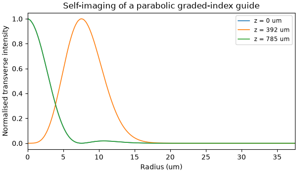
The residual phase after a full turn is the solved spacing’s departure from the ideal one, and nothing else: the guide reproduces its own dispersion, and what is left over is the P1 discretisation of an analytic answer.

entrance = planes[0].field[:, 0, centre]
exit_amplitudes = planes[-1].field[:, 0, centre]
turned = float(
    np.angle((exit_amplitudes[1] / exit_amplitudes[0]) / (entrance[1] / entrance[0]))
)
print(f"residual relative phase {turned:.3e} rad")
predicted = ((solved[0] - solved[1]) - (ideal[0] - ideal[1])) * length
print(f"predicted from the spacing {predicted:.3e} rad")

residual relative phase 5.577e-03 rad
predicted from the spacing 5.577e-03 rad

A launch declared as a field rather than as a channel. The route projects it onto the channels through the record’s coordinate dual and reports what the bound channels did not capture, so a profile the guide cannot carry says so instead of being quietly rescaled.

route = general_modal_route(
    guide, grid, z_max=length, omega_reference=float(grid.omega0)
)
weights = np.array([1.0, 0.5])
declared = np.einsum("qcmw,m->qcw", route.tables.electric[0], weights)
projected = project_transverse_field(route.tables, declared)
print(projected)
ratio = projected.amplitudes[1, centre] / projected.amplitudes[0, centre]
declared_ratio = weights[1] / weights[0]
print(f"amplitude ratio {abs(ratio):.4f} against the declared {declared_ratio}")

ProjectedLaunch: a declared field in a guide's channels
  channels:      2
  frequencies:   65
  peak captured: 1.25 W
  missed share:  1.818e-16
amplitude ratio 0.5000 against the declared 0.5

A field the channels cannot span leaves a remainder, and the projection names it rather than rescaling it away: here the same pattern with its sign flipped on every other node, which is no combination of the two channels at all.

spoiled = declared.copy()
spoiled[::2] *= -1.0
missed = project_transverse_field(route.tables, spoiled).residual_share
print(f"missed share {missed:.3f}")

missed share 1.000

The same happens, less obviously, to a profile declared at one frequency and held across the band: the channels’ patterns change with frequency, so away from where it was declared the field is no longer a guided superposition. The projection reports that too. The share is a reconstruction residual on the guide’s nodes, not radiated power: the energy account of an incident beam is what incident= records (General modal propagation).

held = np.zeros_like(declared)
support = np.any(np.abs(route.tables.electric[0]) > 0.0, axis=(0, 1, 2))
held[:, :, support] = declared[:, :, centre][:, :, None]
held_share = project_transverse_field(route.tables, held).residual_share
print(f"held-profile missed share {held_share:.4f}")

held-profile missed share 0.0286

Related reading

Continue with Radial graded-index fibres for the model, options and limits, and Assessing numerical accuracy for convergence checks. For a paced propagation lesson, return to GNLSE propagation: an N = 3 soliton.