Propagate a vector fibre mode, and check it against the GNLSE

The general modal route propagates a guide’s own three-component E and H (General modal propagation). This example builds a weakly guiding step-index fibre, propagates twenty microns of it with prop_waveguide(provider=...), and compares the self-phase modulation it accumulates with the calibrated GNLSE route at the matched Poynting coefficient.

The comparison is only meaningful because the fibre is weakly guiding: the vector coefficient, which carries the longitudinal field and the |E.E|^2 term, agrees with the scalar n2 omega / (c A_eff) to a fraction of a per cent here. On a sub-micron strand the two differ by a quarter.

import matplotlib.pyplot as plt
import numpy as np

from solprop import fourier
from solprop.constants import C
from solprop.driver import prop_gnlse, prop_waveguide
from solprop.grid import EnvelopeGrid, FieldGrid
from solprop.modes import (
    IndexMaterial,
    MaterialKerr,
    MaterialRegion,
    ModalGuide,
    StepIndexMode,
)
from solprop.nonlinear.normalisation import modal_kerr_coefficient
from solprop.physdata import chi3_from_n2, n2_from_chi3
from solprop.translate.modal_tables import channel_area, sample_modal_table

LENGTH = 2e-5
"""Twenty microns, in about ten accepted steps.

What sets the step here is neither the self-phase modulation nor the general
route: it is the explicit in-stage temporal collar (see "Boundaries" in the model
documentation), whose
rate is set by the length the *grid* was built for, and whose stable step is set
by that rate. A general modal step is expensive, so this example builds its
grids for a millimetre -- a gentle collar -- and propagates twenty microns of it,
to stay inside the documentation build's budget.
"""

WINDOW_LENGTH = 1e-3
"""Length the grids and their collar are declared for, m."""

N2 = 2.6e-20
CHI3 = chi3_from_n2(N2, 1.45)
"""The core's absolute susceptibility, m^2/V^2.

solprop's own conversion, against the core's linear index: a hand-written
``4 eps0 c n^2 n2 / 3`` beside it would be a second copy of the relation.
"""

"The core's absolute susceptibility, m^2/V^2.\n\nsolprop's own conversion, against the core's linear index: a hand-written\n``4 eps0 c n^2 n2 / 3`` beside it would be a second copy of the relation.\n"

The guide: a 4 um core at a 0.01 index step, with the Kerr response declared on the core region and nothing on the cladding, which is how a linear cladding is said to be linear.

grid = FieldGrid.from_limits(WINDOW_LENGTH, 835e-9, (790e-9, 890e-9), 200e-15)
core_law, cladding_law = IndexMaterial(1.45), IndexMaterial(1.44)
mode = StepIndexMode(4e-6, core=1.45, cladding=1.44, profile_wavelength=835e-9)
regions = (
    MaterialRegion("core", 0.0, mode.core_radius, core_law, (MaterialKerr(n2=N2),)),
    MaterialRegion("cladding", mode.core_radius, None, cladding_law),
)
strand = ModalGuide.from_step_index(
    [mode], core=core_law, cladding=cladding_law, regions=regions
).field_provider

# The knots must span the run's whole *active* band, which starts at half the
# lowest declared frequency; the envelope grid below reaches further still, and one
# guide serves both routes.
envelope_grid = EnvelopeGrid.from_limits(
    WINDOW_LENGTH, 835e-9, (790e-9, 890e-9), 200e-15
)
low = min(
    float(grid.omega[grid.active_mask].min()),
    float(envelope_grid.omega[envelope_grid.active_mask].min()),
)
high = max(
    float(grid.omega[grid.active_mask].max()),
    float(envelope_grid.omega[envelope_grid.active_mask].max()),
)
nodes = strand.node_rule(0.99 * low, n_r=24)
guide = ModalGuide.from_provider(
    strand, np.linspace(0.99 * low, 1.01 * high, 13), nodes=nodes
)
print(guide.sampling)

ModalSampling: what a guide's channels were solved on
  knots:         13
  band:          1.048 Prad/s to 2.638 Prad/s
  wavelengths:   714.2 nm to 1.798 um
  position:      0 m
  nodes:         432
  degenerate:    none
  basis:         the provider's own
  profile error: 4.001e-05
  path:          none (a snapshot)

The vector coefficient, and the scalar one the GNLSE would use. metric= is the channel’s own sampled Poynting flux – the metric the route’s projection map contracts with – so the coefficient is the same statement that map makes.

omega0 = float(grid.omega0)
table = sample_modal_table(strand, guide.sampling.omega, np.array([0.0]), nodes)
sample = table.evaluate(omega0, 0.0)
gamma = modal_kerr_coefficient(
    sample.electric[:, :, 0],
    nodes.weights,
    np.where(nodes.region_index == 0, CHI3, 0.0),
    omega0,
    metric=float(np.real(sample.flux_metric[0, 0])),
)
area = channel_area(sample, nodes, 0)
scalar = n2_from_chi3(CHI3, 1.45) * omega0 / (C * area)
print(f"vector gamma {gamma:.6g} 1/(W m), scalar {scalar:.6g} 1/(W m)")
print(f"they differ by {abs(gamma - scalar) / gamma:.2e}")

vector gamma 0.00556005 1/(W m), scalar 0.00555722 1/(W m)
they differ by 5.09e-04

A short run through each route, and each one’s own dispersion-only reference: a guide whose regions declare no response, and gamma = 0.

The general route’s default cubic is the real one, kerr_form="real", which radiates a third harmonic. That is the physical model a field-grid run wants, but it is not what an envelope route carries: prop_gnlse has no room for 3 omega at all. The like-for-like comparison below therefore asks for kerr_form="analytic", the analytic-signal form, which carries the fundamental band alone. The two are one model in two representations and agree for the matched narrowband approximation, up to representation and numerical error — the general modal manual page says why — so what the comparison measures is the two routes and not the choice of form.

linear_guide = ModalGuide.from_provider(
    ModalGuide.from_step_index(
        [mode],
        core=core_law,
        cladding=cladding_law,
        regions=(
            MaterialRegion("core", 0.0, mode.core_radius, core_law),
            MaterialRegion("cladding", mode.core_radius, None, cladding_law),
        ),
    ).field_provider,
    guide.sampling.omega,
    nodes=nodes,
)
common = {
    "lambda0": 835e-9,
    "fwhm": 40e-15,
    "energy": 4e-11,
    "pulseshape": "gauss",
    "n_save": 2,
    "backend": "numpy_ref",
    "progress": "none",
    "dz_max": LENGTH / 10,
    "dz_init": LENGTH / 10,
}
channel = guide.mode_collection.modes[0]
runs = {
    "general": prop_waveguide(
        (), LENGTH, provider=guide, grid=grid, kerr_form="analytic", **common
    ),
    "general, linear": prop_waveguide(
        (), LENGTH, provider=linear_guide, grid=grid, kerr_form="analytic", **common
    ),
    "gnlse": prop_gnlse(
        gamma, LENGTH, grid=envelope_grid, fibre=channel, shock=True, **common
    ),
    "gnlse, linear": prop_gnlse(
        0.0, LENGTH, grid=envelope_grid, fibre=channel, shock=True, **common
    ),
}


def nonlinear_phase(turned, straight, kind):
    """Return the phase the nonlinearity added, against time in the run's frame."""
    a = fourier.inverse(turned.planes()[-1].field[0, 0], kind=kind)
    b = fourier.inverse(straight.planes()[-1].field[0, 0], kind=kind)
    if kind == "field":
        a, b = fourier.analytic_signal(a), fourier.analytic_signal(b)
    keep = np.abs(b) ** 2 > 1e-3 * np.max(np.abs(b) ** 2)
    return keep, np.angle(a[keep] / b[keep]), np.abs(b[keep]) ** 2

/home/docs/checkouts/solprop/checkouts/24/src/solprop/driver/simulation.py:4749: GeneralModalBasisWarning: this general modal guide's interpolated basis is 0.0001136 from orthonormal at 1728.5 nm, above the gram_atol of 0.0001, and that bin is inside the run's active band. The gate this route applies is weighted by the launched spectrum, which discounts that bin to nothing, so it certifies the launch and not the run: a run that broadens into it pays about this much of its physical_energy, because the route declares linear.modal_metric = identity there. The departure is an interpolation error and falls with the knot spacing, so the fix is more knots in the guide's sampling
  route = general_modal_route(
/home/docs/checkouts/solprop/checkouts/24/src/solprop/driver/simulation.py:4749: GeneralModalBasisWarning: this general modal guide's interpolated basis is 0.0001136 from orthonormal at 1728.5 nm, above the gram_atol of 0.0001, and that bin is inside the run's active band. The gate this route applies is weighted by the launched spectrum, which discounts that bin to nothing, so it certifies the launch and not the run: a run that broadens into it pays about this much of its physical_energy, because the route declares linear.modal_metric = identity there. The departure is an interpolation error and falls with the knot spacing, so the fix is more knots in the guide's sampling
  route = general_modal_route(

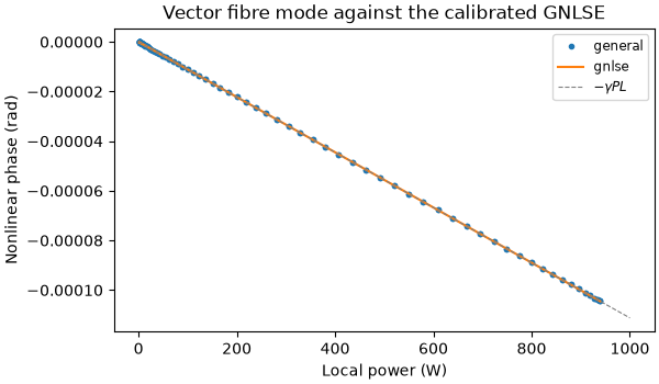
In the internal FFT convention both routes turn by -gamma P(t) L (the public optics-convention phase has the opposite sign), plotted against the local power so that the two grids’ different time samples fall on one curve.

fig, ax = plt.subplots(figsize=(6, 3.5), constrained_layout=True)
for name, kind, style in (
    ("general", "field", {"marker": "o", "linestyle": "none", "markersize": 3}),
    ("gnlse", "envelope", {"linewidth": 1.5}),
):
    _, phase, power = nonlinear_phase(runs[name], runs[f"{name}, linear"], kind)
    order = np.argsort(power)
    ax.plot(power[order], phase[order], label=name, **style)
reference = np.linspace(0.0, 1000.0, 32)
ax.plot(
    reference,
    -gamma * reference * LENGTH,
    color="grey",
    linestyle="--",
    linewidth=0.8,
    label=r"$-\gamma P L$",
)
ax.set(
    xlabel="Local power (W)",
    ylabel="Nonlinear phase (rad)",
    title="Vector fibre mode against the calibrated GNLSE",
)
ax.legend(fontsize="small")
plt.show()

Related reading

Continue with General modal propagation for the model, options and limits, and Assessing numerical accuracy for convergence checks. For a paced propagation lesson, return to GNLSE propagation: an N = 3 soliton.