Note
Go to the end to download the full example code.
Analysing a saved run#
Everything a propagation leaves behind is read through one protocol, and everything drawn from it comes from one set of accessors. This example makes a run without a solver – a Gaussian carried along z by the closed-form phase of pure group-velocity dispersion, which supplies an analytic reference for this example – saves it, reads it back, and draws the standard figures. Swap the synthetic planes for a real output and nothing else changes.
Build the run. A saved plane is a position, a field in the internal FFT convention, and whatever statistics were taken there; a handler stores them and records the grid, the modes and the configuration beside them.
import matplotlib.pyplot as plt
import numpy as np

from solprop.grid import EnvelopeGrid
from solprop.output import MemoryOutput, open_file
from solprop.output.schema import GridRecord, RunMetadata, SavedPlane, StepperRecord
from solprop.plotting import energy, prop_2d, spec_1d, stats, time_1d
from solprop.processing import energy as pulse_energy
from solprop.processing import (
    fwhm_t,
    get_power,
    get_spectral_density,
    grid_of,
    time_bandwidth,
)
from solprop.pulses import GaussianPulse
from solprop.stats import collect, default_spec

LENGTH = 0.2
FWHM = 30e-15

grid = EnvelopeGrid.from_limits(LENGTH, 800e-9, (400e-9, 2e-6), 1e-12)
seed = GaussianPulse(wavelength=800e-9, fwhm=FWHM, energy=1e-6).build(grid)

# Chosen so that the pulse ends four times longer than it started: the closed form is
# tau(z) = tau0 sqrt(1 + (beta2 z / tau0^2)^2) with tau0 the 1/e half-width of the
# field.
tau0 = FWHM / (2 * np.sqrt(np.log(2)))
beta2 = np.sqrt(15) * tau0**2 / LENGTH

metadata = RunMetadata(
    grid=GridRecord.from_grid(grid),
    modes=(),
    simulation_kind="mode_averaged",
    configuration={"beta2": beta2},
    stepper=StepperRecord(tableau="DOPRI5", controller={"rtol": 1e-8}),
)
spec = default_spec("mode_averaged")

run = MemoryOutput()
run.open(metadata)
for z in np.linspace(0.0, LENGTH, 25):
    # The internal linear operator of a purely dispersive co-moving frame.
    field = seed * np.exp(-0.5j * beta2 * (grid.omega - grid.omega0) ** 2 * z)
    plane = SavedPlane(z=float(z), field=field)
    run.save(SavedPlane(z=float(z), field=field, stats=collect(spec, grid, plane)))

print(f"{run.n_saved} planes on a {grid.kind} grid of {grid.n_omega} bins")
25 planes on a envelope grid of 1024 bins
Read it back. The accessors take the handler, not the grid: they rebuild the axes from the metadata, return the active band on an ascending axis, and squeeze the mode and polarisation axes a mode-averaged run does not need.
wavelength, density = get_spectral_density(run, "wavelength", plane=-1)
t, power = get_power(run, plane=-1, oversampling=4)

print(f"axes: {wavelength.shape} wavelengths, {t.shape} time samples")
print(f"energy {float(pulse_energy(run, plane=-1)) * 1e6:.4f} uJ")
print(f"duration {float(fwhm_t(run, plane=-1)) * 1e15:.1f} fs")
print(f"time-bandwidth product {float(time_bandwidth(run, plane=-1)):.3f}")
axes: (853,) wavelengths, (4096,) time samples
energy 1.0000 uJ
duration 120.0 fs
time-bandwidth product 1.766
The metrics against the closed form. Pure dispersion conserves the energy and the spectrum exactly and stretches the pulse by a known factor, so the measured duration is a check on the whole chain: the stored convention, the rebuilt axes, the transform and the half-maximum crossing.
z = run["z"]
measured = fwhm_t(run)
expected = FWHM * np.sqrt(1.0 + (beta2 * z / tau0**2) ** 2)

fig, ax = plt.subplots(figsize=(5.6, 3.2))
ax.plot(z * 100, measured * 1e15, lw=3, alpha=0.4, label="measured")
ax.plot(
    z * 100,
    expected * 1e15,
    "k--",
    lw=1,
    label=r"$\tau_0\sqrt{1+(\beta_2z/\tau_0^2)^2}$",
)
ax.set_xlabel("distance (cm)")
ax.set_ylabel("duration (fs)")
ax.legend(frameon=False)
fig.tight_layout()

print(f"largest relative error {np.max(np.abs(measured / expected - 1)):.2e}")
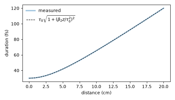
largest relative error 2.66e-04
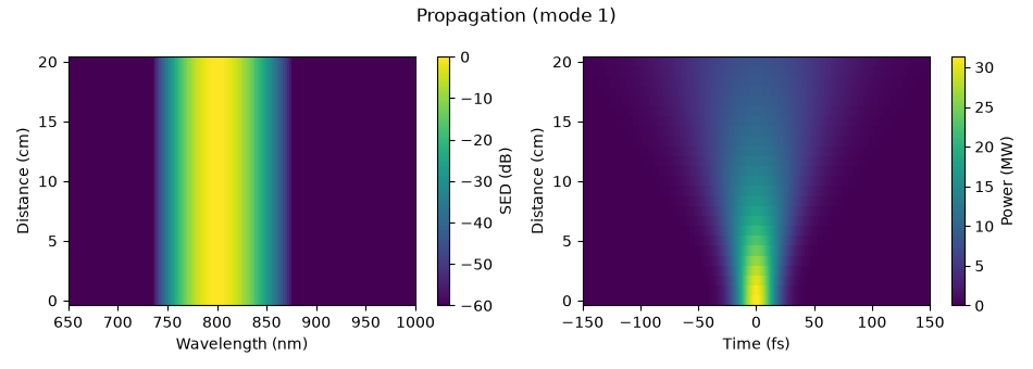
The propagation maps. One figure per mode and one for the modal sum; here there is one mode, so there is one figure. The spectral panel is in decibels below the peak and the temporal one is a linear power in an auto-chosen unit.
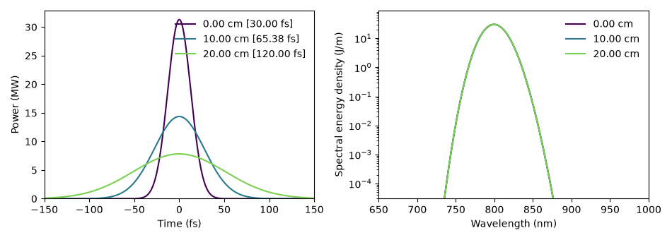
Slices at three positions. A colour per position; the temporal legend carries each trace’s width at half maximum, and the spectral axis is logarithmic over six decades by default.
fig, (left, right) = plt.subplots(1, 2, figsize=(9.5, 3.4))
time_1d(run, [0.0, 0.1, 0.2], trange=(-150e-15, 150e-15), ax=left)
spec_1d(run, [0.0, 0.1, 0.2], wavelength_range=(650e-9, 1000e-9), ax=right)
fig.tight_layout()
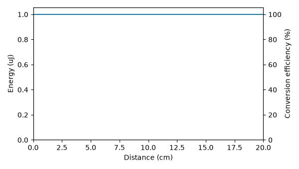
The energy along the fibre, with the conversion efficiency on the right-hand axis. Pure dispersion moves neither, which is the point: a plot that shows nothing happening is how you find out that nothing happened.
figure = energy(run)
figure.set_size_inches(6.0, 3.4)
figure.tight_layout()
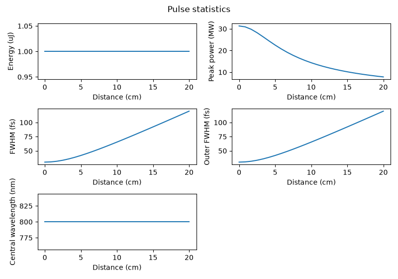
The statistics the run recorded. Only the groups with something in them are drawn, so a run that recorded no waveguide statistics gets one figure rather than an error.
figure = stats(run)[0]
figure.set_size_inches(8.0, 5.6)
figure.tight_layout()
The same run from disk. A memory handler writes exactly the file the HDF5 handler
would have written, open_file opens it again read-only through the same protocol,
and an accessor reading either returns the same bits – which is what makes it safe
to develop an analysis against a small in-memory run and then point it at a large
file.
import tempfile
from pathlib import Path

with tempfile.TemporaryDirectory() as directory:
    path = Path(directory) / "run.h5"
    run.to_file(path, compression="lzf")
    with open_file(path) as from_disk:
        same_grid = grid_of(from_disk).n_omega == grid.n_omega
        _, from_file = get_spectral_density(from_disk, "wavelength", plane=-1)
    print(f"grid rebuilt from the file: {same_grid}")
    print(f"densities identical: {np.array_equal(density, from_file)}")
grid rebuilt from the file: True
densities identical: True