Note
Go to the end to download the full example code.
Spatiotemporal propagation in a graded-index multimode fibre#
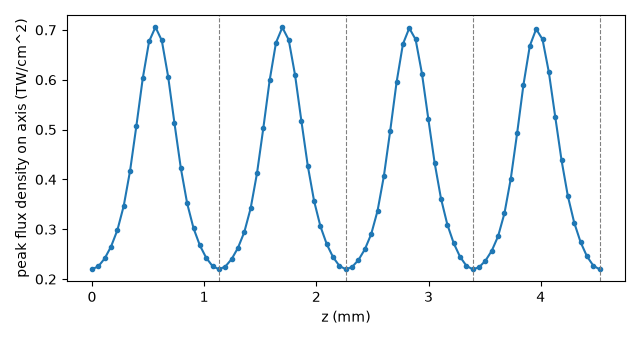
A parabolic graded-index fibre provides a useful setting for studying periodic transverse motion and nonlinear spectral broadening. Its mode groups are almost equally spaced in propagation constant, so a beam launched into several of them self-images: the transverse pattern contracts and expands with a period of a fraction of a millimetre, and the intensity on the axis oscillates with it. At high power that periodic oscillation is a longitudinal grating written into the Kerr effect, and it phase-matches geometric parametric instability (GPI): sidebands far from the pump, with the leading-order, weak-nonlinearity estimate for frequency offsets \(\Omega_h = \sqrt{2\pi h/(z_p\beta_2)}\), where \(z_p\) is the self-imaging period and \(\beta_2\) the group-velocity dispersion (Krupa et al., Phys. Rev. Lett. 116, 183901 (2016), doi:10.1103/PhysRevLett.116.183901; Wright et al., Nat. Photon. 9, 306 (2015)).
This example propagates that system on the general modal route
(General modal propagation): a
GradedIndexProvider solves the fibre’s own
fields at every frequency across the band, the run synthesises the physical field at
the guide’s quadrature nodes, evaluates the silica core’s Kerr response there –
including its third harmonic – and projects it back onto the channels. Nothing is
reduced to an effective area or a table of overlap integrals.
The fibre is a 100 um core (50 um radius), parabolic, index contrast \(\Delta = 0.0095\) (a numerical aperture of 0.2), on dispersive fused silica. The pump is a 300 fs pulse at 1064 nm with 500 kW peak power – well below the critical power for self-focusing, about 4 MW – carried by a centred Gaussian beam of 12 um waist, declared as an incident beam and coupled into the fibre’s channels under the vector paraxial model (Coupling simulations).
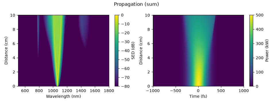
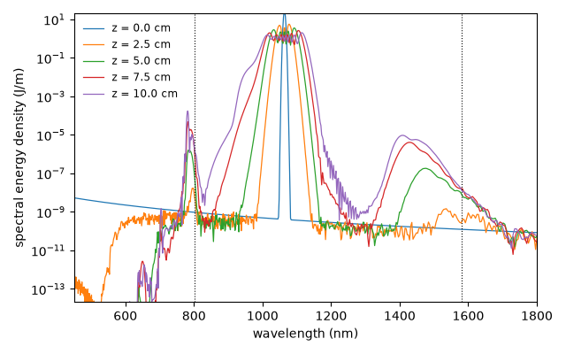
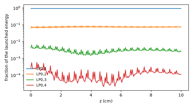
What to look for. The on-axis intensity oscillates at the self-imaging period from the entrance; the spectrum grows sidebands near the GPI frequencies predicted from that period and the silica dispersion; the energy the launch put in each channel is redistributed by the nonlinearity.
What is approximate, and what was chosen. A centred beam excites only the
radially symmetric modes, so the guide is the weak-guidance LP_0m family (the
provider’s scalar approximation, whose contrast limit this fibre is inside); four
of them, because the guide must be solved over the run’s whole active band, which
reaches 3.6 um, and a fifth LP_0m channel is not bound there. The beam’s
peak power and energy are those of the whole incident beam; the run launches only
the share of it the four channels capture – light they miss would be lost at the
entrance, not restored – and the coupling report gives both energies. A 12 um beam
is close to the fibre’s fundamental mode (about 9 um), so the four LP_0m
channels take all but a few parts in \(10^5\) of it. This is a truncated
model, not a mode-count convergence study. The quadrature
uses two angular nodes, exact for fields with no azimuthal dependence. Raman
scattering is left out, to keep the run to minutes: a silica core would declare
SilicaTensorResponse beside its Kerr term. The
self-imaging period is set by the finite-element solve of the parabolic core, whose
propagation constants converge at second order in the element count.
The fibre#
The core law is fused silica’s Sellmeier fit (Malitson’s, optmat’s absolute
malitson_1965/sellmeier reached by its former name) on the axis, scaled by
the parabola; the cladding is the same glass scaled by 1 - 2 Delta, written as
a small permittivity law of our own – anything with permittivity,
omega_domain and identity is one
(PermittivityLaw). The core declares its Kerr
response by \(n_2\), at the wavelength it was measured.
import time
from dataclasses import dataclass

import matplotlib.pyplot as plt
import numpy as np

from solprop.constants import C
from solprop.coupling import CouplingModel
from solprop.driver import prop_waveguide
from solprop.grid import FieldGrid
from solprop.modes import (
    GradedIndexProvider,
    IndexMaterial,
    MaterialKerr,
    ModalGuide,
    PowerLawPermittivity,
)
from solprop.physdata import fused_silica
from solprop.plotting import prop_2d
from solprop.processing import get_spectral_density
from solprop.processing.modal import physical_energy, reconstructed_flux
from solprop.pulses import GaussianPulse, SpatialPulse
from solprop.translate.general import general_modal_route

RADIUS = 50e-6
"""Core radius, m."""

DELTA = 0.0095
"""Index contrast: eps(r) = eps_axis (1 - 2 Delta (r/a)^2) in the core."""

WAVELENGTH = 1.064e-6
"""Pump wavelength, m."""

LENGTH = 0.1
"""Fibre length, m."""

WAIST = 12e-6
"""1/e field (1/e^2 intensity) radius of the incident Gaussian beam, m."""

PEAK_POWER = 5e5
"""Peak power of the whole incident beam, W."""

FWHM = 300e-15
"""Incident duration, s."""

started = time.perf_counter()
silica = IndexMaterial(fused_silica(model="malitson_1965/sellmeier"))


@dataclass(frozen=True)
class ScaledPermittivity:
    """A permittivity law multiplied by a constant factor."""

    law: IndexMaterial
    factor: float

    def permittivity(self, omega):
        return self.factor * self.law.permittivity(omega)

    @property
    def omega_domain(self):
        return self.law.omega_domain

    @property
    def identity(self):
        return {"law": dict(self.law.identity), "factor": self.factor}


provider = GradedIndexProvider(
    permittivity=PowerLawPermittivity(silica, DELTA),
    exterior=ScaledPermittivity(silica, 1.0 - 2.0 * DELTA),
    radius=RADIUS,
    family="LP",
    count=4,
    elements=64,
    extent=1.6,
    core_responses=(MaterialKerr(n2=2.7e-20, at=WAVELENGTH),),
)
print(provider)
GradedIndexProvider: radial P1 elements, exact Bessel exterior
  sector:        LP0
  approximation: weak-guidance LP
  channels:      4
  radius:        50 um
  elements:      64
  extent:        1.6 core radii
  exterior:      ScaledPermittivity
The grid spans 450 nm to 1.8 um, which holds both GPI sidebands, and 1.2 ps. The guide is solved at 97 frequencies across the active band – from half the grid’s lowest declared frequency, 3.6 um, to its highest – on a node rule of two Gauss points per radial element and two angular nodes. The route gates the interpolated basis’s departure from orthonormality where the launched pulse is, and would warn if it exceeded its budget anywhere else in the active band; this guide’s sampling passes without a warning.
grid = FieldGrid.from_limits(LENGTH, WAVELENGTH, (450e-9, 1.8e-6), 1.2e-12)
active = grid.omega[grid.active_mask]
nodes = provider.node_rule(0.99 * float(active[0]), n_r=2, n_theta=2)
guide = ModalGuide.from_provider(
    provider,
    np.geomspace(0.99 * float(active[0]), 1.01 * float(active[-1]), 97),
    nodes=nodes,
)
print(guide)
print(f"{grid.n_omega} frequency bins, {nodes.xy.shape[0]} quadrature nodes")
ModalGuide: a mode collection and its full-vector provider
  provider: GradedIndexProvider(LP0, 4 channels, 64 elements, extent=1.6)
  channels: LP0,1, LP0,2, LP0,3, LP0,4
  regions:  core (MaterialKerr(n2=2.7e-20 m^2/W, at 1.064 um)), exterior
  sampling: ModalSampling(97 knots, 519 Trad/s to 4.648 Prad/s, 412 nodes)
2049 frequency bins, 412 quadrature nodes
The channels and the self-imaging period. For an ideal infinite parabola the
LP_0m propagation constants are equally spaced by 2 sqrt(2 Delta)/a, so
the pattern repeats every z_p = pi a / sqrt(2 Delta). The solved spacings of
the finite, dispersive fibre are close to that and not equal to it.
centre = int(np.argmin(np.abs(grid.omega - grid.omega0)))
neff = np.array(
    [
        mode.neff(grid.omega[centre : centre + 1])[0].real
        for mode in guide.mode_collection.modes
    ]
)
beta = neff * float(grid.omega[centre]) / C
spacing = -np.diff(beta)
ideal = 2.0 * np.sqrt(2.0 * DELTA) / RADIUS
z_p = 2.0 * np.pi / float(np.mean(spacing))
labels = [label.display_label for label in guide.mode_collection.channel_labels]
print(
    "effective indices:",
    ", ".join(f"{name} {value:.7f}" for name, value in zip(labels, neff, strict=True)),
)
print(f"spacings {np.array2string(spacing, precision=1)} 1/m; ideal {ideal:.1f} 1/m")
print(
    f"self-imaging period z_p = {z_p * 1e3:.4f} mm "
    f"(ideal {np.pi * RADIUS / np.sqrt(2 * DELTA) * 1e3:.4f} mm)"
)
effective indices: LP0,1 1.4495475, LP0,2 1.4486103, LP0,3 1.4476691, LP0,4 1.4467240
spacings [5530.3 5553.5 5576.7] 1/m; ideal 5513.6 1/m
self-imaging period z_p = 1.1314 mm (ideal 1.1396 mm)
The run#
prop_waveguide(..., provider=guide, incident=beam, coupling=...). The beam is
a SpatialPulse: a Gaussian of the 12 um waist, centred
on the axis and polarised along x, carrying the 300 fs pulse; its energy is the
whole beam’s, over its own plane. The run couples it into the four channels under
the vector paraxial model – the flux pairing of the beam’s field, with the forward
paraxial closure for its magnetic field, against the channels’ own E/H at the
nodes – whose admission budget, model_error, bounds that closure’s error,
the guide’s contrast and the angular content of the beam and channels. The
recovered amplitudes are launched unscaled: the launched energy is the share of
the incident energy the channels capture, and anything they miss is lost at the
entrance. model_error=0.1 admits this guide: the weak-guidance contrast,
0.0095, must stay below an eighth of the budget, and the counted terms (printed
below) sum to about 0.02.
Shot noise is added to the input (noise="input", one photon per bin and
channel, with a fixed seed), because GPI grows from noise at frequencies the pump
does not contain. dz_max is a tenth of the self-imaging period: the source
oscillates at that period, and the adaptive stepper would otherwise try steps that
straddle it. The default cubic is the real one, so the third harmonic is carried
too.
beam = SpatialPulse(
    GaussianPulse(
        wavelength=WAVELENGTH,
        fwhm=FWHM,
        energy=PEAK_POWER * FWHM * np.sqrt(np.pi / (4.0 * np.log(2.0))),
    ),
    WAIST,
)
coupling = CouplingModel("vector_paraxial", model_error=0.1)


def propagate(length, n_save):
    """Propagate the incident beam through `length` of the fibre."""
    return prop_waveguide(
        (),
        length,
        provider=guide,
        grid=grid,
        incident=beam,
        coupling=coupling,
        lambda0=WAVELENGTH,
        noise="input",
        seed=41,
        dz_max=z_p / 10.0,
        n_save=n_save,
        progress="none",
    )


run = propagate(LENGTH, 201)
print(run)
MemoryOutput
  state:           closed
  planes:          201, 0 m to 100 mm
  field per plane: 4 x 1 x 2049 (modes x components x omega)
  statistics:      analytic_flux, fwhm_t, fwhm_t_outer, omega0, physical_energy
  between planes:  none
  run:             RunMetadata(multimode, field grid of 4096, 4 modes, native, 2026-1...
The launch account#
The run records the coupling’s report as configuration["launch"]: the
incident energy over the beam’s whole plane, the energy the channels launch, the
captured energy where the model defines one, and the admission budget against
model_error. The vector model names no captured or uncaptured energy – the
flux pairing and the incident measure are not one positive metric – so its
launched share is the measure of what the four channels take: here all but a
few parts in \(10^5\), mostly in LP_01. The launched energy is what the
run’s physical_energy reads at the entrance.
launch = run.metadata.configuration["launch"]
print(launch)
captured = launch.captured_energy
print(
    f"incident {launch.incident_energy * 1e9:.2f} nJ, "
    f"launched {launch.launched_energy * 1e9:.2f} nJ "
    f"({launch.efficiency:.5f} of the incident energy), captured "
    + (
        f"{captured * 1e9:.2f} nJ"
        if captured is not None
        else f"not defined ({launch.captured_reason})"
    )
)
print(f"admission budget {launch.budget:.3e} of model_error {launch.model_error:g}")
entrance = np.sum(np.abs(np.asarray(run["field"])[0, :, 0, :]) ** 2, axis=-1)
print(
    "launched shares:",
    ", ".join(
        f"{name} {share:.3f}"
        for name, share in zip(labels, entrance / entrance.sum(), strict=True)
    ),
)
CouplingReport: a field coupled into an input port
  model:          vector_paraxial
  incident:       159.7 nJ
  launched:       159.7 nJ
  launched share: 1.0000 of the incident energy
  uncaptured:     not defined
  budget:         1.832e-02 of model_error 0.1
  angular:        1.250e-02 (field) incident field: cone-rule allocation (1 - cos the...
  numerical:      0.000e+00 (field) source domain/resolution 0.0e+00, field beyond th...
  source metric:  9.473e-05 (field) common measure M0 against the plane's native metric
  target metric:  2.517e-08 (map) F at the port's nodes against the native Q
  contrast:       9.500e-03 (model) weak-guidance screen Delta over the guide's regions
  closure:        4.617e-03 (map) H_t = Y0 z x E_t against provider H, field error 2....
  angular:        0.000e+00 (map) retained target subspace: cone-rule allocation (1 -...
  envelope:       n/a (model) no recorded pair envelope: omitted facet reflection is ...
  passivity:      1.107e-03 (field) apparent gain within the model's defects, reporte...
  exterior:       zero
incident 159.67 nJ, launched 159.67 nJ (0.99998 of the incident energy), captured not defined (vector_paraxial recovers coordinates with the flux pairing F; F and the incident measure M0 are not one positive metric, so no orthogonal remainder is a physical loss (section 4.3))
admission budget 1.832e-02 of model_error 0.1
launched shares: LP0,1 0.933, LP0,2 0.062, LP0,3 0.004, LP0,4 0.000
Self-imaging#
The ten-centimetre run saves a plane every half millimetre, which is too sparse
to show the shape of a pattern that repeats every 1.13 mm, so the first four periods
are
run again
with twenty planes per period. The flux density at the nodes nearest the axis,
peaked over time, is rebuilt from the saved channel amplitudes and the guide’s own
fields (solprop.processing.modal.reconstructed_flux() with density=True),
which is why the guide and its tables are passed beside the output. The dashed
lines mark the period the channels’ spacings predict. The launch is mostly
LP_01 with a few per cent of LP_02, so what oscillates is their beat.
imaging = propagate(4.0 * z_p, 81)
imaging_route = general_modal_route(
    guide, grid, z_max=4.0 * z_p, omega_reference=float(grid.omega0)
)
radius = np.hypot(nodes.xy[:, 0], nodes.xy[:, 1])
axis_nodes = radius <= np.min(radius) * 1.0001
z_imaging = np.asarray(imaging["z"])
on_axis = np.array(
    [
        np.max(
            np.mean(
                reconstructed_flux(
                    imaging, imaging_route.tables, plane=i, density=True, guide=guide
                )[axis_nodes],
                axis=0,
            )
        )
        for i in range(z_imaging.size)
    ]
)
fig, ax = plt.subplots(figsize=(6.4, 3.4))
ax.plot(z_imaging * 1e3, on_axis * 1e-4 * 1e-12, "o-", markersize=3)
for period in range(1, 5):
    ax.axvline(period * z_p * 1e3, color="0.5", linestyle="--", linewidth=0.8)
ax.set_xlabel("z (mm)")
ax.set_ylabel("peak flux density on axis (TW/cm^2)")
fig.tight_layout()
The spectrum#
The propagation map first, summed over the channels: the pump broadens by self-phase modulation, and two bands far from it grow out of the noise floor: a narrow one near 785 nm from about 4 cm, and a broader one near 1.45 um from about 5.5 cm. The pulse spreads in time as it goes, because self-phase modulation in normal dispersion broadens it.
z = np.asarray(run["z"])
figures = prop_2d(
    run,
    "wavelength",
    wavelength_range=(500e-9, 1.8e-6),
    trange=(-1e-12, 1e-12),
    db_min=-80,
    modes="sum",
)
figures[-1].set_size_inches(9.5, 3.6)
figures[-1].tight_layout()
The spectral energy density summed over the channels, at the entrance and every
2.5 cm, on a logarithmic scale, with the first GPI sideband pair predicted from
z_p and the group-velocity dispersion of bulk silica at the pump (the fibre’s
waveguide contribution to it is small for a core this large).
The anti-Stokes band sits within 2 % of the predicted 802 nm – close agreement
for a formula that keeps only beta_2 across a 90 THz shift. The long-wavelength
band is not at the predicted Stokes position (1.58 um), nor at the
energy-conserving partner of the anti-Stokes band (1.64 um); the leading-order
formula does not explain it, and this page leaves it as an open observation.
omega0 = 2.0 * np.pi * C / WAVELENGTH
index = fused_silica(model="malitson_1965/sellmeier")
step = omega0 * 1e-3
beta = np.array(
    [
        np.real(index.index(np.array([w]))[0]) * w / C
        for w in (omega0 - step, omega0, omega0 + step)
    ]
)
beta2 = float((beta[0] - 2.0 * beta[1] + beta[2]) / step**2)
shift = np.sqrt(2.0 * np.pi / (z_p * beta2))
sidebands = [2.0 * np.pi * C / (omega0 + sign * shift) for sign in (1.0, -1.0)]
print(f"silica beta2 at the pump {beta2 * 1e27:.2f} fs^2/mm")
print(
    f"predicted first GPI pair: {sidebands[0] * 1e9:.0f} nm "
    f"and {sidebands[1] * 1e9:.0f} nm"
)

fig, ax = plt.subplots(figsize=(6.4, 4.0))
for position in (0.0, 0.025, 0.05, 0.075, 0.1):
    plane = int(np.argmin(np.abs(z - position)))
    wavelength, density = get_spectral_density(
        run, "wavelength", plane=plane, modes="sum"
    )
    order = np.argsort(wavelength)
    ax.semilogy(
        wavelength[order] * 1e9,
        density[order],
        linewidth=0.9,
        label=f"z = {z[plane] * 100:.1f} cm",
    )
for line in sidebands:
    ax.axvline(line * 1e9, color="k", linestyle=":", linewidth=0.8)
ax.set_xlim(450.0, 1800.0)
ax.set_ylim(1e-14 * np.max(density), 10.0 * np.max(density))
ax.set_xlabel("wavelength (nm)")
ax.set_ylabel("spectral energy density (J/m)")
ax.legend(frameon=False, fontsize="small")
fig.tight_layout()
silica beta2 at the pump 16.53 fs^2/mm
predicted first GPI pair: 802 nm and 1582 nm
The channels#
The energy in each channel along the fibre, as a fraction of the launched
energy, on a logarithmic scale. On the provider’s own basis the channels are
orthonormal in true power, so a channel’s energy is the frequency sum of its own
|a|^2 and the four add to the route’s physical_energy (printed). The
small, fast ripple is the Kerr exchange between the channels at the beat period;
the slow drift is what the nonlinearity moves over centimetres.
field = np.asarray(run["field"])[:, :, 0, :]
per_channel = np.sum(np.abs(field) ** 2, axis=-1)
fraction = per_channel / per_channel[0].sum()
fig, ax = plt.subplots(figsize=(6.4, 3.6))
for channel, name in enumerate(labels):
    ax.semilogy(z * 100, fraction[:, channel], label=name)
ax.set_xlabel("z (cm)")
ax.set_ylabel("fraction of the launched energy")
ax.legend(frameon=False, fontsize="small")
fig.tight_layout()

print(
    f"physical energy: {float(physical_energy(run, plane=0)) * 1e9:.2f} nJ in, "
    f"{float(physical_energy(run, plane=-1)) * 1e9:.2f} nJ out"
)
for position, index in (("entrance", 0), ("exit", -1)):
    text = ", ".join(
        f"{name} {share:.2e}"
        for name, share in zip(labels, fraction[index], strict=True)
    )
    print(f"{position:8s}: {text}")
physical energy: 159.67 nJ in, 159.68 nJ out
entrance: LP0,1 9.33e-01, LP0,2 6.25e-02, LP0,3 4.13e-03, LP0,4 2.75e-04
exit    : LP0,1 9.28e-01, LP0,2 6.95e-02, LP0,3 2.46e-03, LP0,4 1.10e-04
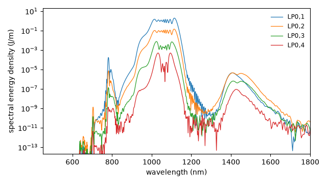
Which channel carries which band: the exit spectrum of each channel. The pump
stays mostly in LP_01; the bands the parametric process built are shared
between the channels, because the process that made them is the beat between
the channels.
wavelength, densities = get_spectral_density(run, "wavelength", plane=-1)
order = np.argsort(wavelength)
fig, ax = plt.subplots(figsize=(6.4, 3.6))
for channel, name in enumerate(labels):
    ax.semilogy(
        wavelength[order] * 1e9, densities[channel][order], linewidth=0.9, label=name
    )
ax.set_xlim(450.0, 1800.0)
ax.set_ylim(1e-14 * np.max(densities), 10.0 * np.max(densities))
ax.set_xlabel("wavelength (nm)")
ax.set_ylabel("spectral energy density (J/m)")
ax.legend(frameon=False, fontsize="small")
fig.tight_layout()
Runtime and reproducibility#
A ten-centimetre and a 4.5 mm run of four channels on the general modal route.
623 s; backend native, 18 threads