A tapered graded-index fibre: adiabatic and abrupt mode conversion

A fibre taper changes the shape of the modes it guides. In a parabolic graded-index core the fundamental mode is, to a very good approximation, a Gaussian whose width squared is proportional to the core radius, \(w^2 = 2a/(k n_1 \sqrt{2\Delta})\); narrow the core from 25 um to 15 um and the mode narrows by \(\sqrt{0.6}\). If the core narrows slowly, the light follows the local mode and stays in it – the taper is adiabatic. If it narrows quickly, the light keeps the shape it had, which is no longer a mode of the narrower core, and part of it is left in the next mode that shares its symmetry, LP_02. The rule of thumb that separates the two is Love’s: a taper is adiabatic where its local length scale \(z_t = a/|da/dz|\) is longer than the beat length \(z_b = 2\pi/(\beta_1 - \beta_2)\) between the two modes (J. D. Love et al., IEE Proc. J 138, 343 (1991); T. A. Birks and Y. W. Li, J. Lightwave Technol. 10, 432 (1992)).

This example propagates such tapers on the moving solid guide of the general modal route (General modal guides that vary along the propagation). The guide is a GradedIndexProvider whose core radius follows a Linear or PiecewiseLinear path. The route re-solves the fibre’s fields along that path, so that the synthesis and projection maps – which put the Kerr response on the fields of the core where the pulse is – move with the modes, and it carries the connection \(\langle\psi_m|\partial_z\psi_n \rangle\) between the channels in its frozen-section flow. It is the connection that converts LP_01 into LP_02; an effective-area model, or a guide held at its entrance shape, has nothing that could.

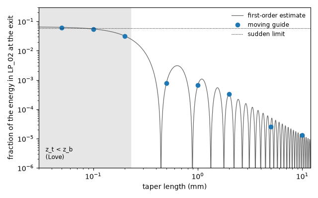
The fibre has a 25 um core radius and an index contrast \(\Delta = 0.0095\) (a numerical aperture of 0.2), tapered linearly to 15 um. The pump is at 1030 nm. First the linear problem: eight taper lengths from 50 um to 10 mm, at a picojoule, with the conversion each leaves in LP_02 compared with a first-order coupled-mode estimate and with Love’s criterion; then the fields of the channels at the entrance and at the waist of an abrupt taper, rebuilt from the run. Last, a 400 kW, 200 fs pulse through a slow taper followed by a 10 mm waist, where self-phase modulation grows as the mode area shrinks, against the scalar SpecifiedMode model of the same fibre, against a one-channel moving guide, and against the fibre held at its entrance radius.

What to look for. The conversion falls from several per cent for the shortest tapers to 1e-5 for the longest, as the square of the taper slope, with the oscillation in length a two-ended conversion makes; the estimate from the connection and the beat length tracks it wherever it is small, and the shortest taper approaches the sudden limit, a splice between the two cores. 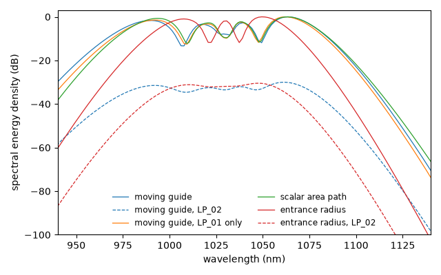Along the slow taper LP_02 beats at the beat length about a level set by the taper’s slope; the abrupt taper’s waist field carries LP_02’s ring. In the nonlinear run the spectrum broadens more than the entrance guide allows, by the mode’s own shrinking area; the one-channel moving guide and the scalar area path agree, because this taper is adiabatic; and the two-channel guide broadens 5 % more than either, because at 9 % of the critical power the Kerr effect narrows the beam itself – a self-focusing lens that, on the modes, is an LP_02 admixture.

What is approximate. The provider solves the weak-guidance scalar LP sector, exact to leading order in \(\Delta\) (vector corrections omitted), and only its two lowest radial channels are carried: LP_01 couples to LP_02 alone in an infinite parabola (the derivative of a Gaussian’s width is the next Laguerre-Gauss mode), and LP_02’s own coupling to LP_03 enters only at second order. The Kerr lens is carried only as far as two radial channels can describe a narrowing beam: the agreement shown at 9 % of the estimated critical power is with a variational Gaussian model, not a mode-count convergence study, and does not establish accuracy near collapse. The material is a constant index of 1.45: over these lengths a 200 fs pulse’s dispersion length in silica is metres, and a Sellmeier core would cost the guide’s solves a factor of three. The flow freezes the modes’ departure at each section’s midpoint and carries the rest in the explicit residual, so its step is limited by the spread of the channels’ propagation constants across a section (the run’s advisory step, which dz_max respects here). The collar absorber at the grid’s edges is the default. No Raman response is declared.

The fibre

The core law is the parabola PowerLawPermittivity on a constant index; the cladding is the same index scaled by 1 - 2 Delta. The Kerr response is declared on the core by its \(n_2\). taper_guide builds the guide for any radius path: the provider owns the path, and from_provider() samples it along z, at the Chebyshev degree its own held-out check demands, as well as at the frequency knots.

import time
import warnings

import matplotlib.pyplot as plt
import numpy as np
from scipy.interpolate import CubicSpline

from solprop.constants import C
from solprop.driver import Simulation, prop_gnlse, prop_waveguide
from solprop.exceptions import GeneralModalBasisWarning
from solprop.grid import EnvelopeGrid, FieldGrid
from solprop.modes import (
    GradedIndexProvider,
    IndexMaterial,
    MaterialKerr,
    ModalGuide,
    PowerLawPermittivity,
)
from solprop.modes.connection import modal_connection
from solprop.nonlinear.gnlse import SpecifiedMode
from solprop.processing import get_spectral_density
from solprop.processing.modal import coordinate_intensity, reconstructed_flux
from solprop.profiles import Linear, PiecewiseLinear
from solprop.translate.coupled import advisory_step
from solprop.translate.general import general_modal_route
from solprop.translate.modal_path import path_rule

ENTRANCE = 25e-6
"""Core radius at the entrance, m."""

WAIST = 15e-6
"""Core radius at the taper's waist, m."""

DELTA = 0.0095
"""Index contrast: eps(r) = eps_axis (1 - 2 Delta (r/a)^2) in the core."""

WAVELENGTH = 1.03e-6
"""Pump wavelength, m."""

N2 = 2.7e-20
"""Nonlinear index of the core, m^2/W."""

DZ_MAX = 1.2e-4
"""Longest step, m: below the flow's advisory step, which the run prints (see below)."""

started = time.perf_counter()
core = IndexMaterial(1.45)
cladding = IndexMaterial(1.45 * np.sqrt(1.0 - 2.0 * DELTA))


def taper_guide(radius, grid, knots=17, count=2):
    """Return the graded-index guide's ``LP_0m`` channels on a radius path."""
    provider = GradedIndexProvider(
        permittivity=PowerLawPermittivity(core, DELTA),
        exterior=cladding,
        radius=radius,
        family="LP",
        count=count,
        elements=48,
        extent=2.0,
        core_responses=(MaterialKerr(n2=N2, at=WAVELENGTH),),
    )
    active = grid.omega[grid.active_mask]
    frequencies = np.geomspace(0.99 * float(active[0]), 1.01 * float(active[-1]), knots)
    return ModalGuide.from_provider(
        provider,
        frequencies,
        nodes=provider.node_rule(float(frequencies[0]), 0.0, n_r=2, n_theta=2),
    )


def linear_grid(length):
    """Return the narrow grid the picojoule runs propagate on."""
    return FieldGrid.from_limits(length, WAVELENGTH, (1.0e-6, 1.065e-6), 0.4e-12)


reference_length = 1e-3
reference = taper_guide(Linear(ENTRANCE, WAIST, reference_length), linear_grid(1e-3))
print(reference)
print(reference.sampling.path)

ModalGuide: a mode collection and its full-vector provider
  provider: GradedIndexProvider(LP0, 2 channels, 48 elements, extent=2)
  channels: LP0,1, LP0,2
  regions:  core (MaterialKerr(n2=2.7e-20 m^2/W, at 1.03 um)), exterior
  sampling: ModalSampling(17 knots, 885.1 Trad/s to 2.085 Prad/s, 384 nodes)
ModalPath: how a moving guide was sampled along z
  sections:       1 (1 per kink interval)
  span:           0 m to 1 mm
  degree:         8
  positions:      9
  budget:         2.446e-06
  held-out error: 3.143e-07
  gram departure: 1.335e-06

How fast is too fast

Two numbers decide it at every position: the connection \(\Gamma_{21}\), how fast LP_01 turns into LP_02 as the core narrows, and the splitting \(\beta_1 - \beta_2\), how fast the two drift out of phase. Both are measured here from the provider directly – the connection by modal_connection(), a difference of fresh solves, and the propagation constants by fresh solves – along the 1 mm reference taper, at the pump frequency. For an infinite parabola \(\Gamma_{21} = a'/(2a)\) exactly (the width \(w \propto \sqrt a\)) and \(\beta_1 - \beta_2 = 2\sqrt{2\Delta}/a\), so their ratio \(a'/(4\sqrt{2\Delta})\) does not change along a linear taper, and Love’s ratio \(z_t/z_b\) is \(\sqrt{2\Delta}/(\pi |a'|)\), the same at every position. The finite fibre, with its cladding, is within a part in a thousand of both (the sign of \(\Gamma_{21}\) is the provider’s choice of the modes’ signs).

provider = reference.field_provider
omega0 = 2.0 * np.pi * C / WAVELENGTH
positions = np.linspace(0.0, 1.0, 65)
connection = np.empty(positions.size)
splitting = np.empty(positions.size)
for i, fraction in enumerate(positions):
    z = fraction * reference_length
    connection[i] = np.real(modal_connection(provider, omega0, z).matrix[1, 0])
    rule = provider.node_rule(omega0, z, n_r=2, n_theta=2)
    beta = np.real(1j * np.diag(provider.solve(omega0, z, nodes=rule).generator))
    splitting[i] = beta[0] - beta[1]
slope = (WAIST - ENTRANCE) / reference_length
radius_along = ENTRANCE + slope * positions * reference_length
for i in (0, 32, 64):
    print(
        f"a = {radius_along[i] * 1e6:4.1f} um: Gamma_21 = {connection[i]:7.1f} 1/m "
        f"(ideal {abs(slope) / (2.0 * radius_along[i]):7.1f}), "
        f"beta_1 - beta_2 = {splitting[i]:7.1f} 1/m "
        f"(ideal {2.0 * np.sqrt(2.0 * DELTA) / radius_along[i]:7.1f}), "
        f"beat length {2.0 * np.pi / splitting[i] * 1e3:.3f} mm"
    )
love_length = abs(WAIST - ENTRANCE) * np.pi / np.sqrt(2.0 * DELTA)
print(f"Love's criterion z_t = z_b at a taper length of {love_length * 1e3:.3f} mm")

a = 25.0 um: Gamma_21 =   200.2 1/m (ideal   200.0), beta_1 - beta_2 = 11065.2 1/m (ideal 11027.2), beat length 0.568 mm
a = 20.0 um: Gamma_21 =   250.2 1/m (ideal   250.0), beta_1 - beta_2 = 13829.8 1/m (ideal 13784.0), beat length 0.454 mm
a = 15.0 um: Gamma_21 =   333.5 1/m (ideal   333.3), beta_1 - beta_2 = 18441.3 1/m (ideal 18378.7), beat length 0.341 mm
Love's criterion z_t = z_b at a taper length of 0.228 mm

The first-order estimate. Launched in LP_01, the amplitude left in LP_02 after a taper of length \(L\) is, while it is small,

\[b_2(L) \approx -\int_0^L \Gamma_{21}(z)\, e^{i\int_0^z (\beta_1 - \beta_2)\,dz'} \,dz .\]

On a linear taper of any length the connection is the reference’s scaled by 1 mm / L at the same fraction of the taper, and the splitting is the same, so one set of measurements gives the estimate for every length; both are smooth, and are interpolated by cubic splines onto the fine grid the phase needs at 10 mm. At the ends of the taper the slope jumps, and the integrand’s two ends are where the conversion is made: the two contributions interfere, which is the oscillation in length. The sudden limit is the other end: a taper so short that the field does not change at all, a splice, leaves \(|c_1|^2 = (2 w_0 w_1/(w_0^2+w_1^2))^2 ((w_0^2 - w_1^2)/(w_0^2 + w_1^2))^2\) in LP_02 (the overlap of one Gaussian with the other’s first radial Laguerre-Gauss mode).

fine = np.linspace(0.0, 1.0, 20001)
fine_connection = CubicSpline(positions, connection)(fine)
phase = CubicSpline(positions, splitting).antiderivative()(fine)


def first_order(length):
    """Return the estimated ``LP_02`` amplitude along a taper of `length`."""
    integrand = fine_connection * reference_length * np.exp(1j * length * phase)
    steps = 0.5 * (integrand[1:] + integrand[:-1]) * np.diff(fine)
    return np.concatenate(([0.0], np.cumsum(steps)))


ratio = WAIST / ENTRANCE
sudden = (2.0 * np.sqrt(ratio) / (1.0 + ratio)) ** 2 * (
    (1.0 - ratio) / (1.0 + ratio)
) ** 2
print(f"sudden limit (a splice from 25 um to 15 um): {sudden:.4f} of the power")

sudden limit (a splice from 25 um to 15 um): 0.0586 of the power

The linear conversion

Eight tapers from 50 um to 10 mm long, each launched with a 100 fs, 1 pJ pulse in LP_01 – weak enough to isolate linear conversion in this comparison. Each channel’s energy at a plane is the frequency sum of its own \(|b|^2\): the channels are orthonormal in true power at every position, so the two add to the run’s physical energy. dz_max holds every step below the advisory step the translation computes, \(0.9/K\), with \(K\) the spread of the channels’ propagation constants about a section’s midpoint over the bins the error norm scores (the only ones the explicit residual is applied on). It does not depend on the taper’s length, because the radius changes by the same amount whatever the length; the run prints it for the longest taper below. The two channels together keep the launched energy to about 1e-6 in every run.

lengths = np.array([0.05, 0.1, 0.2, 0.5, 1.0, 2.0, 5.0, 10.0]) * 1e-3


def channel_fractions(run):
    """Return the positions and each channel's energy over the launched energy."""
    field = np.asarray(run["field"])[:, :, 0, :]
    energy = np.sum(np.abs(field) ** 2, axis=-1)
    return np.asarray(run["z"]), energy / energy[0].sum()


linear_runs = {}
for length in lengths:
    grid = linear_grid(length)
    guide = taper_guide(Linear(ENTRANCE, WAIST, length), grid)
    run = prop_waveguide(
        (),
        length,
        provider=guide,
        grid=grid,
        lambda0=WAVELENGTH,
        fwhm=100e-15,
        energy=1e-12,
        dz_max=min(DZ_MAX, length / 10.0),
        n_save=41,
        progress="none",
    )
    linear_runs[length] = (guide, grid, run)
    z, fractions = channel_fractions(run)
    print(
        f"L = {length * 1e3:5.2f} mm: LP_02 holds {fractions[-1, 1]:.3e} at the exit "
        f"(first order {abs(first_order(length)[-1]) ** 2:.3e}); "
        f"energy lost {1.0 - fractions[-1].sum():.1e}"
    )

grid = linear_grid(lengths[-1])
problem = Simulation.from_waveguide(
    (),
    lengths[-1],
    provider=linear_runs[lengths[-1]][0],
    grid=grid,
    lambda0=WAVELENGTH,
    fwhm=100e-15,
    energy=1e-12,
    dz_max=DZ_MAX,
).translate()
flow = problem.linear.coupled_flow
assert flow is not None
advisory = float(np.min(advisory_step(flow, problem.grids.inband_mask)))
print(f"advisory step {advisory * 1e3:.3f} mm against dz_max {DZ_MAX * 1e3:.3f} mm")

L =  0.05 mm: LP_02 holds 6.131e-02 at the exit (first order 6.267e-02); energy lost 8.1e-07
L =  0.10 mm: LP_02 holds 5.394e-02 at the exit (first order 5.517e-02); energy lost 8.2e-07
L =  0.20 mm: LP_02 holds 3.112e-02 at the exit (first order 3.192e-02); energy lost 8.5e-07
L =  0.50 mm: LP_02 holds 7.900e-04 at the exit (first order 7.597e-04); energy lost 1.1e-06
L =  1.00 mm: LP_02 holds 6.548e-04 at the exit (first order 6.496e-04); energy lost 1.1e-06
L =  2.00 mm: LP_02 holds 3.271e-04 at the exit (first order 3.272e-04); energy lost 8.3e-07
L =  5.00 mm: LP_02 holds 2.525e-05 at the exit (first order 2.520e-05); energy lost 1.2e-06
L = 10.00 mm: LP_02 holds 1.307e-05 at the exit (first order 1.307e-05); energy lost 1.3e-06
advisory step 0.130 mm against dz_max 0.120 mm

The conversion at the exit against the taper’s length. The dots are the runs; the line is the first-order estimate, with its oscillation, and the dotted line the sudden limit; the shaded region is where Love’s criterion calls the taper non-adiabatic. From 0.5 mm up the runs sit on the estimate to within 4 % of the conversion, down to 1.3e-5 at 10 mm, where the exit happens to land near a maximum of the oscillation. Below Love’s length the estimate overshoots, as it does in this case: at zero length it gives \((\int\Gamma_{21}dz)^2 = (\ln(w_1/w_0))^2\) = 0.065 against the sudden limit’s 0.059, and the runs lie between the two, approaching the splice.

dense = np.geomspace(0.03e-3, 12e-3, 3000)
fig, ax = plt.subplots(figsize=(6.4, 4.0))
ax.loglog(
    dense * 1e3,
    [abs(first_order(length)[-1]) ** 2 for length in dense],
    color="0.4",
    linewidth=0.9,
    label="first-order estimate",
)
ax.loglog(
    lengths * 1e3,
    [channel_fractions(linear_runs[length][2])[1][-1, 1] for length in lengths],
    "o",
    label="moving guide",
)
ax.axhline(sudden, color="k", linestyle=":", linewidth=0.8, label="sudden limit")
ax.axvspan(dense[0] * 1e3, love_length * 1e3, color="0.9", zorder=0)
ax.text(0.035, 2e-6, "z_t < z_b\n(Love)", fontsize="small")
ax.set_xlim(dense[0] * 1e3, dense[-1] * 1e3)
ax.set_ylim(1e-6, 0.3)
ax.set_xlabel("taper length (mm)")
ax.set_ylabel("fraction of the energy in LP_02 at the exit")
ax.legend(frameon=False, fontsize="small", loc="upper right")
fig.tight_layout()

An abrupt and a slow taper

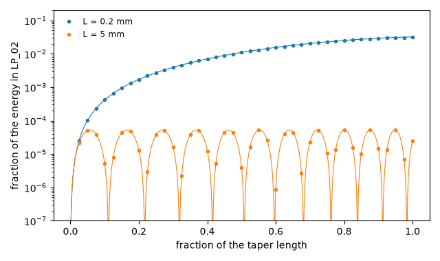
Along the taper, against its fraction of the length: the 0.2 mm taper (Love’s ratio 0.9) and the 5 mm one (22), with the first-order estimate beside each. The abrupt taper is shorter than one beat length (0.34 to 0.57 mm), so its LP_02 grows steadily across it, a splice spread over 0.2 mm. On the slow taper the entrance, where the slope jumps from zero, leaves an amplitude \(\Gamma_{21}/(\beta_1 - \beta_2) = a'/(4\sqrt{2\Delta})\), 3.6e-3, which then beats against the same amplitude the local modes carry while the core narrows: the power swings between nothing and \(4(a'/(4\sqrt{2\Delta}))^2\) = 5e-5 once per beat length, and the exit, where the slope returns to zero, keeps what it finds there. Every point of the run is on the estimate.

fig, ax = plt.subplots(figsize=(6.4, 3.8))
for length, colour in ((0.2e-3, "C0"), (5e-3, "C1")):
    z, fractions = channel_fractions(linear_runs[length][2])
    ax.semilogy(
        z / length,
        np.maximum(fractions[:, 1], 1e-12),
        "o",
        markersize=3,
        color=colour,
        label=f"L = {length * 1e3:g} mm",
    )
    ax.semilogy(
        fine,
        np.maximum(np.abs(first_order(length)) ** 2, 1e-12),
        color=colour,
        linewidth=0.8,
    )
ax.set_ylim(1e-7, 0.2)
ax.set_xlabel("fraction of the taper length")
ax.set_ylabel("fraction of the energy in LP_02")
ax.legend(frameon=False, fontsize="small")
fig.tight_layout()

The fields

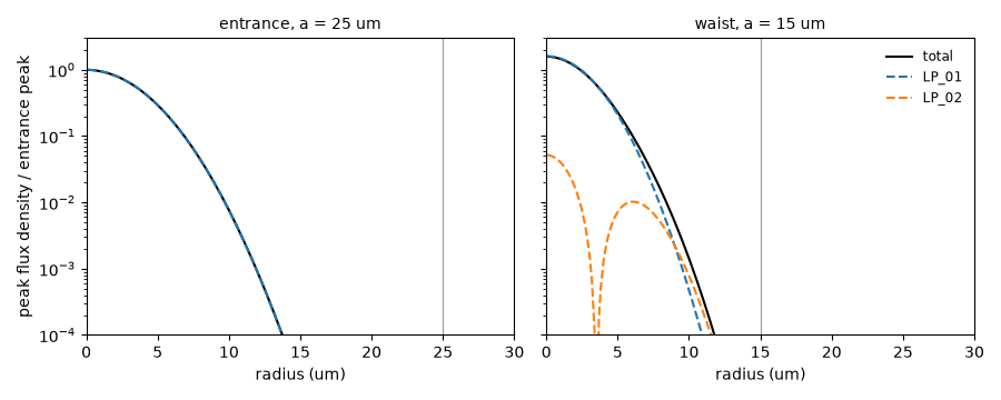
The abrupt taper’s field at its entrance and at its waist, rebuilt from the run’s saved channel amplitudes and the guide’s own fields at each plane’s position: the accessors of solprop.processing.modal solve the guide again there, on the node rule that has moved with the core, so the waist plane is reconstructed on the waist’s modes and nodes. The flux density (reconstructed_flux() with density=True) and each channel’s own share (coordinate_intensity()) are peaked over time and plotted against the radius, relative to the entrance’s peak. The waist’s LP_01 is narrower and 1.6 times as intense: the area ratio, 1.67, less the 3 % the taper moved out of it; LP_02, with its node at 3.5 um and its ring outside it, is what the abrupt narrowing left behind (at the entrance it is empty and off the scale). The grey line is the core’s edge; the fields have fallen by four decades well inside it.

guide, grid, run = linear_runs[0.2e-3]
with warnings.catch_warnings():
    warnings.simplefilter("ignore", GeneralModalBasisWarning)
    tables = general_modal_route(
        guide, grid, z_max=0.2e-3, omega_reference=float(grid.omega0)
    ).tables
fig, axes = plt.subplots(1, 2, figsize=(9.0, 3.6), sharey=True)
peak = None
for ax, plane, title in (
    (axes[0], 0, "entrance, a = 25 um"),
    (axes[1], -1, "waist, a = 15 um"),
):
    z = float(np.asarray(run["z"])[plane])
    nodes = path_rule(guide.field_provider, guide.sampling.nodes, z)
    radius = np.hypot(nodes.xy[:, 0], nodes.xy[:, 1])
    order = np.argsort(radius)
    total = np.max(
        reconstructed_flux(run, tables, plane=plane, density=True, guide=guide), axis=-1
    )
    channels = np.max(
        coordinate_intensity(run, tables, plane=plane, guide=guide), axis=-1
    )
    if peak is None:
        peak = float(np.max(total))
    ax.semilogy(radius[order] * 1e6, total[order] / peak, color="k", label="total")
    for channel, name in enumerate(("LP_01", "LP_02")):
        ax.semilogy(
            radius[order] * 1e6,
            np.maximum(channels[channel][order] / peak, 1e-30),
            linestyle="--",
            label=name,
        )
    ax.axvline(
        float(guide.field_provider.radius(np.array([z]))[0]) * 1e6,
        color="0.6",
        linewidth=0.8,
    )
    ax.set_title(title, fontsize="medium")
    ax.set_xlabel("radius (um)")
    ax.set_xlim(0.0, 30.0)
axes[0].set_ylabel("peak flux density / entrance peak")
axes[0].set_ylim(1e-4, 3.0)
axes[1].legend(frameon=False, fontsize="small")
fig.tight_layout()

Self-phase modulation in a taper’s waist

A 200 fs, 400 kW pulse through a 5 mm taper, adiabatic by a factor of 22 on Love’s criterion, and a 10 mm waist. The Kerr term is the analytic one, which carries the fundamental band only, so that the envelope model below is a like-for-like comparison. Four runs:

• the moving guide, two channels, which puts the Kerr response on the fields of the core where the pulse is and projects it back onto both;

• the same moving guide with one channel, LP_01 alone;

• the scalar model of the same fibre: prop_gnlse with a SpecifiedMode carrying the guide’s own LP_01 dispersion along z (from_mode()) and the effective area along the taper, measured from the provider’s fields at the pump wavelength, so that \(\gamma(z) = n_2\omega_0/(c A(z))\); it moves the area but not the modes, and could not convert;

• the fibre held at its entrance radius, a guide that does not move at all.

The effective area of the ideal parabola is proportional to the radius, so a path that is linear between the taper’s corners is exact for it; the printed mid-taper value checks that on the real fibre. The peak power is 9 % of the critical power for self-focusing, \(P_{cr} = \lambda^2/(2\pi n_0 n_2)\) in the Gaussian-beam estimate (printed), which matters below.

LENGTH = 15e-3
CORNER = 5e-3
WINDOW = (0.93e-6, 1.15e-6)
PULSE = {"lambda0": WAVELENGTH, "fwhm": 200e-15, "peak_power": 4e5}
path = PiecewiseLinear(
    np.array([0.0, CORNER, LENGTH]), np.array([ENTRANCE, WAIST, WAIST])
)
field_grid = FieldGrid.from_limits(LENGTH, WAVELENGTH, WINDOW, 2e-12)
envelope_grid = EnvelopeGrid.from_limits(LENGTH, WAVELENGTH, WINDOW, 2e-12)
moving_guide = taper_guide(path, field_grid, knots=25)
single_guide = taper_guide(path, field_grid, knots=25, count=1)
still_guide = taper_guide(ENTRANCE, field_grid, knots=25)


def effective_area(guide, z):
    """Return ``LP_01``'s effective area at the pump, m^2, from a fresh solve."""
    source = guide.field_provider
    rule = source.node_rule(omega0, z, n_r=2, n_theta=2)
    field = source.solve(omega0, z, nodes=rule).electric[:, :, 0]
    density = np.sum(np.abs(field) ** 2, axis=1)
    weights = rule.weights
    return float(np.sum(weights * density) ** 2 / np.sum(weights * density**2))


areas = [effective_area(moving_guide, z) for z in (0.0, 0.5 * CORNER, CORNER)]
print(
    "effective area: "
    f"{areas[0] * 1e12:.1f} um^2 at the entrance, {areas[2] * 1e12:.1f} um^2 in the "
    f"waist; mid-taper {areas[1] * 1e12:.2f} um^2 against the linear path's "
    f"{0.5 * (areas[0] + areas[2]) * 1e12:.2f}"
)
gamma = [N2 * omega0 / (C * area) for area in areas]
phase_moving = PULSE["peak_power"] * (
    0.5 * (gamma[0] + gamma[2]) * CORNER + gamma[2] * (LENGTH - CORNER)
)
phase_still = PULSE["peak_power"] * gamma[0] * LENGTH
print(
    f"gamma {gamma[0] * 1e3:.3f} /(W km) at the entrance, "
    f"{gamma[2] * 1e3:.3f} in the waist"
)
print(
    f"peak nonlinear phase: {phase_moving:.1f} rad through the taper, "
    f"{phase_still:.1f} rad at the entrance radius"
)
critical = WAVELENGTH**2 / (2.0 * np.pi * 1.45 * N2)
lens = 1.0 / np.sqrt(1.0 - PULSE["peak_power"] / critical)
print(
    f"critical power {critical * 1e-6:.2f} MW; P/P_cr = "
    f"{PULSE['peak_power'] / critical:.3f}; the Kerr lens raises the peak's "
    f"coefficient by {lens:.4f}"
)

common = {"n_save": 31, "progress": "none", **PULSE}
moving = prop_waveguide(
    (),
    LENGTH,
    provider=moving_guide,
    grid=field_grid,
    kerr_form="analytic",
    dz_max=DZ_MAX,
    **common,
)
single = prop_waveguide(
    (),
    LENGTH,
    provider=single_guide,
    grid=field_grid,
    kerr_form="analytic",
    dz_max=DZ_MAX,
    **common,
)
area_path = PiecewiseLinear(
    np.array([0.0, CORNER, LENGTH]), np.array([areas[0], areas[2], areas[2]])
)
scalar = prop_gnlse(
    None,
    LENGTH,
    grid=envelope_grid,
    fibre=SpecifiedMode.from_mode(
        moving_guide.mode_collection.modes[0], aeff=area_path
    ),
    n2=N2,
    shock=True,
    backend="numba_cpu",
    **common,
)
still = prop_waveguide(
    (), LENGTH, provider=still_guide, grid=field_grid, kerr_form="analytic", **common
)

effective area: 129.0 um^2 at the entrance, 77.3 um^2 in the waist; mid-taper 103.14 um^2 against the linear path's 103.15
gamma 1.277 /(W km) at the entrance, 2.130 in the waist
peak nonlinear phase: 11.9 rad through the taper, 7.7 rad at the entrance radius
critical power 4.31 MW; P/P_cr = 0.093; the Kerr lens raises the peak's coefficient by 1.0499

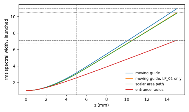
The spectral width of LP_01 along the fibre. The rms width of a Gaussian pulse’s spectrum grows with the peak nonlinear phase \(\phi\) as \(\sqrt{1 + 4\phi^2/(3\sqrt3)}\) (G. P. Agrawal, Nonlinear Fiber Optics, section 4.1), dispersion aside; the dotted lines are that growth for the two phases printed above. The taper’s runs grow faster from the start and end well above the fibre held at its entrance radius, by the area ratio. The one-channel moving guide and the scalar area path end on their dotted line, together (the first is under the second): on an adiabatic taper, moving the modes and moving the area are the same physics.

The two-channel runs end 5 % above their lines, taper and entrance guide alike. That is the Kerr lens: at 9 % of the critical power the beam’s own index change narrows it, and in a parabolic core a Gaussian beam’s area at power \(P\) is its linear area times \(\sqrt{1 - P/P_{cr}}\); the dashed lines are the Gaussian law with the peak’s phase raised by that factor. A narrower LP_01-like beam is, on the fibre’s modes, LP_01 with a little LP_02 in phase with it – which is how the two-channel route carries it, and why a model with one field shape, however it moves along z, cannot. The width is taken on LP_01 alone, since an rms width weights far wings by the square of their distance.

def rms_width(run, plane):
    """Return the rms width of ``LP_01``'s spectrum at a plane, rad/s."""
    omega, density = get_spectral_density(run, "omega", plane=plane, modes=0)
    omega, density = np.asarray(omega), np.ravel(density)
    mean = np.sum(omega * density) / np.sum(density)
    return float(np.sqrt(np.sum((omega - mean) ** 2 * density) / np.sum(density)))


nonlinear_runs = (
    (moving, "moving guide"),
    (single, "moving guide, LP_01 only"),
    (scalar, "scalar area path"),
    (still, "entrance radius"),
)
COLOURS = ("C0", "C1", "C2", "C3")
fig, ax = plt.subplots(figsize=(6.4, 3.8))
for (run, name), colour in zip(nonlinear_runs, COLOURS, strict=True):
    z = np.asarray(run["z"])
    widths = np.array([rms_width(run, plane) for plane in range(z.size)])
    ax.plot(z * 1e3, widths / widths[0], color=colour, label=name)
    print(f"{name:24s}: LP_01 rms spectral width x{widths[-1] / widths[0]:.3f}")
for phase_end in (phase_moving, phase_still):
    for factor, style in ((1.0, ":"), (lens, "--")):
        expected = np.sqrt(1.0 + 4.0 * (factor * phase_end) ** 2 / (3.0 * np.sqrt(3.0)))
        print(f"Gaussian SPM at {factor * phase_end:.2f} rad: x{expected:.3f}")
        ax.axhline(expected, color="0.5", linestyle=style, linewidth=0.8)
ax.axvline(CORNER * 1e3, color="0.6", linestyle="--", linewidth=0.8)
ax.set_xlabel("z (mm)")
ax.set_ylabel("rms spectral width / launched")
ax.legend(frameon=False, fontsize="small")
fig.tight_layout()

moving guide            : LP_01 rms spectral width x10.988
moving guide, LP_01 only: LP_01 rms spectral width x10.487
scalar area path        : LP_01 rms spectral width x10.433
entrance radius         : LP_01 rms spectral width x7.144
Gaussian SPM at 11.92 rad: x10.510
Gaussian SPM at 12.52 rad: x11.030
Gaussian SPM at 7.66 rad: x6.798
Gaussian SPM at 8.05 rad: x7.130

The spectra at the exit, in decibels below the LP_01 peak of each run, with the two-channel runs’ LP_02 dashed. The LP_01 spectra of the taper’s runs share their long-wavelength edge; the two-channel run’s short-wavelength lobe reaches further, as its larger phase requires. Its LP_02 is 30 dB down and has the pump’s own self-phase shape, which is what a Kerr lens looks like on the modes: a cross term the pump writes wherever it is intense, not a band of its own. The taper by itself converts 2.5e-5 at this length (above); the printed LP_02 share is fifty times that, and nearly the same in the fibre that does not taper at all.

fig, ax = plt.subplots(figsize=(6.4, 4.0))
for (run, name), colour in zip(nonlinear_runs, COLOURS, strict=True):
    wavelength, density = get_spectral_density(run, "wavelength", plane=-1)
    density = np.asarray(density).reshape(-1, np.size(wavelength))
    order = np.argsort(wavelength)
    reference_peak = float(np.max(density[0]))
    for channel, style in enumerate(("-", "--")[: density.shape[0]]):
        ax.plot(
            np.asarray(wavelength)[order] * 1e9,
            10.0
            * np.log10(np.maximum(density[channel][order] / reference_peak, 1e-12)),
            style,
            color=colour,
            linewidth=0.9,
            label=name if channel == 0 else f"{name}, LP_02",
        )
ax.set_xlim(940.0, 1140.0)
ax.set_ylim(-100.0, 3.0)
ax.set_xlabel("wavelength (nm)")
ax.set_ylabel("spectral energy density (dB)")
ax.legend(frameon=False, fontsize="small", loc="lower center", ncol=2)
fig.tight_layout()

for run, name in ((moving, "moving guide"), (still, "entrance radius")):
    z, fractions = channel_fractions(run)
    print(f"{name}: LP_02 holds {fractions[-1, 1]:.2e} of the energy at the exit")

moving guide: LP_02 holds 1.30e-03 of the energy at the exit
entrance radius: LP_02 holds 1.26e-03 of the energy at the exit

Runtime and reproducibility

Twelve guides, eight linear runs on the moving guide and four nonlinear runs.

settings = moving.metadata.backend.settings
print(
    f"{time.perf_counter() - started:.0f} s; backend {moving.metadata.backend.name}, "
    f"{settings.get('thread_count', 'default')} threads"
)

195 s; backend native, 18 threads

Related reading

Continue with General modal guides that vary along the propagation for the model, options and limits, and Assessing numerical accuracy for convergence checks. For a paced introduction to propagation, start with the Introduction.