Separate nitrogen and oxygen ionisation in an air-filled capillary

A 15 um radius, 0.225 m capillary contains dry air at 6 bar and 300 K. The 800 nm input has 30 fs intensity FWHM and 2.2 uJ energy. Nitrogen and oxygen each take optmat’s recommended molecular rate (plasma by label), and deplete independently under their shared electric field. Argon contributes dispersion and Kerr response but has no ionisation channel in this example.

The reduced mode-averaged grid keeps this gallery calculation short. It is an interface and bookkeeping example, not a converged ultraviolet prediction. The 300 nm to 2 um grid lies inside optmat’s refractivity fits (N2 from 145 nm, O2 from 195 nm, Ar from 107.5 nm, each to the static limit), but at 6 bar the mixture’s Raman response is used above its validated density, and the run warns about it (MaterialRangeWarning). This example selects nitrogen’s Raman bands only; raman=True would add oxygen’s. The response is optmat’s for the composition: its linewidths follow the summed density of the broadening partners, and each band’s amplitude its own population.

from time import perf_counter

import matplotlib.pyplot as plt
import numpy as np

from solprop.driver import Simulation, SimulationSettings
from solprop.grid import FieldGrid
from solprop.modes import MarcatiliMode
from solprop.nonlinear import responses_for
from solprop.physdata import Mixture
from solprop.processing import species_ionisation, species_ionisation_energy
from solprop.pulses import GaussianPulse
from solprop.stats import StatsSpec
from solprop.stepper import PIController

One material declaration feeds the linear operator and every nonlinear channel. The default fractions are divided by 0.9996 because carbon dioxide is omitted.

started = perf_counter()
mixture = Mixture.air(6.0, temperature=300.0)
# The weak entrance ionisation has narrow sub-cycle rate peaks. The ionisation
# quadrature
# resolves their local contribution without enlarging the coarse spectral state;
# sampling and step convergence remain separate checks.
grid = FieldGrid.from_limits(0.225, 800e-9, (300e-9, 2e-6), 200e-15, ffac=24.0)
mode = MarcatiliMode(15e-6, mixture=mixture, loss=True, cladding=1.45)
responses = responses_for(
    mixture,
    plasma={"N2": True, "O2": True},
    raman=("N2",),
    thg=False,
    lambda0=800e-9,
)
simulation = Simulation(
    grid,
    mode,
    responses,
    GaussianPulse(wavelength=800e-9, fwhm=30e-15, energy=2.2e-6),
    settings=SimulationSettings(
        controller=PIController(rtol=1e-5, atol=1e-12),
        save_planes=np.linspace(0.0, grid.length, 21)[1:],
        dz_init=1e-5,
        dz_max=2e-3,
        ionisation_field_range=(1e7, 1e12),
        stats=StatsSpec(
            names=(
                "energy",
                "species_ionisation",
                "species_electron_density",
                "species_peak_ionisation_rate",
                "species_density",
                "species_ionisation_energy",
            )
        ),
    ),
)
run = simulation.run()
z = run["z"]
fractions = species_ionisation(run)
inventory = species_ionisation_energy(run)

/home/docs/checkouts/solprop/checkouts/24/src/solprop/nonlinear/optmat_raman.py:1121: MaterialRangeWarning: N2+O2+Ar: optmat's Raman response raman_response/N2+O2+Ar@300K,800nm is used outside its validated density range (5.396 to 5.396 amagat). optmat: density above 2.07 amagat, where the lines overlap: their mixing is not modelled (TC-527, TC-688)
  densities = _check_range(response, request)

These are inventories at the end of each local pulse. With preionisation, pulse source increments would subtract rho_s f0_s, and pulse work would subtract the corresponding initial ionisation energy. This example starts neutral.

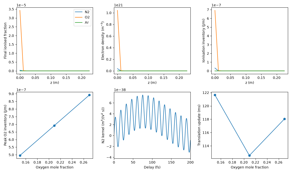
figure, axes = plt.subplots(2, 3, figsize=(12, 7))
for index, label in enumerate(mixture.labels):
    axes[0, 0].plot(z, fractions[:, index, 0], label=label)
    axes[0, 1].plot(z, run["stats/species_electron_density"][:, index], label=label)
    axes[0, 2].plot(z, inventory[:, index], label=label)
axes[0, 0].set(ylabel="Final ionised fraction", xlabel="z (m)")
axes[0, 1].set(ylabel="Electron density (m$^{-3}$)", xlabel="z (m)")
axes[0, 2].set(ylabel="Ionisation inventory (J/m)", xlabel="z (m)")
_ = axes[0, 0].legend()

Replacing oxygen with nitrogen keeps total pressure and the small argon fraction fixed. Changing fractions changes the pressure-dependent operator function, so with_mixture rebuilds those coefficients while sharing rates, geometry and input.

oxygen = np.array([0.15, mixture.fractions[1], 0.27])
oxygen_inventory = []
update_seconds = []
for fraction in oxygen:
    composition = {
        "N2": 1.0 - fraction - mixture.fractions[2],
        "O2": float(fraction),
        "Ar": mixture.fractions[2],
    }
    before = perf_counter()
    changed = simulation.with_mixture(mixture.with_fill(composition))
    update_seconds.append(perf_counter() - before)
    result = changed.run()
    oxygen_inventory.append(float(np.max(species_ionisation_energy(result)[:, 1])))
axes[1, 0].plot(oxygen, oxygen_inventory, "o-")
_ = axes[1, 0].set(xlabel="Oxygen mole fraction", ylabel="Peak O2 inventory (J/m)")

The nitrogen kernel combines all its sampled terms with the entrance linewidth. Its units follow P_R(t) = eps0 rho_N2 E(t) integral h(t-t’) E(t’)^2 dt’.

leaf = simulation.translate().responses.raman_terms[0]
delay = np.arange(leaf.undamped.shape[-1]) * grid.dt_fine
rates = np.array([float(table(0.0)) for table in leaf.decay_rates])
kernel = np.sum(leaf.undamped * np.exp(-rates[:, None] * delay), axis=0)
axes[1, 1].plot(delay * 1e15, kernel)
axes[1, 1].set(xlabel="Delay (fs)", ylabel="N2 kernel (m$^5$/(V$^2$ s))", xlim=(0, 200))
axes[1, 2].plot(oxygen, np.array(update_seconds) * 1e3, "o-")
axes[1, 2].set(xlabel="Oxygen mole fraction", ylabel="Translation update (ms)")
figure.tight_layout()
print("Oxygen Raman omitted by the explicit raman=('N2',) selection.")
print(f"with_mixture translation times (s): {update_seconds}")
print(f"Complete example and three-point sweep: {perf_counter() - started:.3f} s")

Oxygen Raman omitted by the explicit raman=('N2',) selection.
with_mixture translation times (s): [0.1216349190000301, 0.1125484609999603, 0.11803526000005604]
Complete example and three-point sweep: 11.815 s

Related reading

Continue with Gas mixtures for the model, options and limits, and Assessing numerical accuracy for convergence checks. For a paced propagation lesson, return to Resonant dispersive-wave propagation.