A hollow planar waveguide, per unit width#

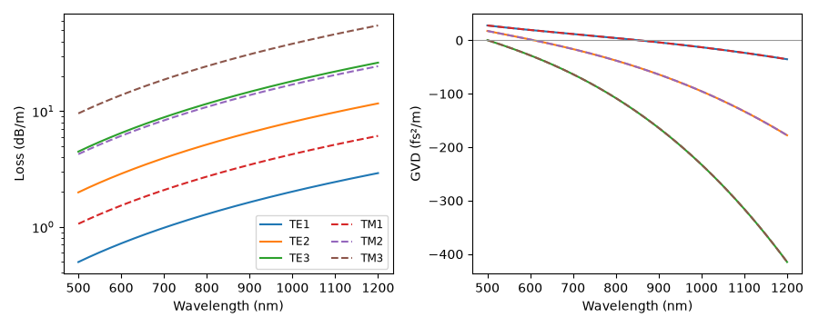
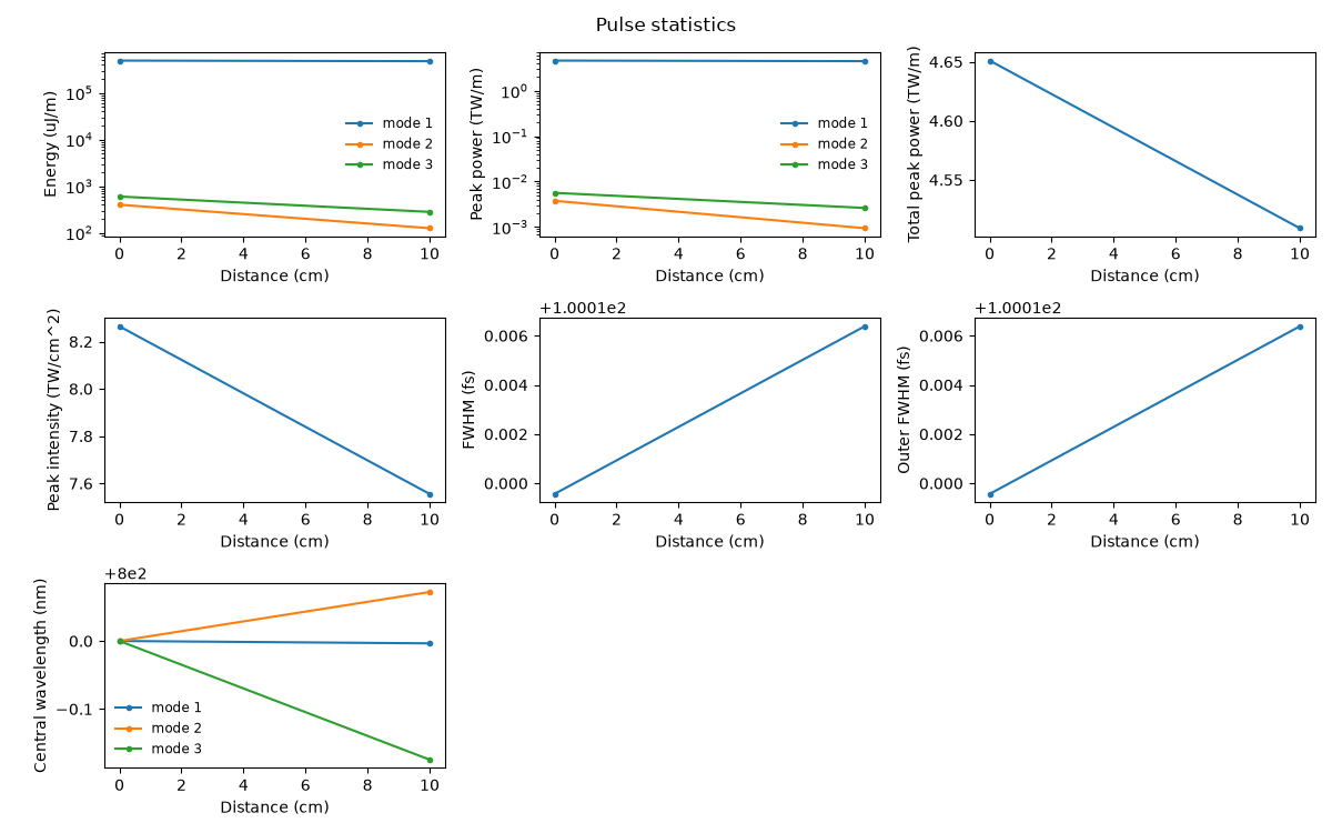
Two silica plates 127 um apart, filled with argon: the planar compressor of Akturk et al. (2009). The guide is modelled uniform in y – a plane wave in the free direction – so every power is per metre of y (W/m) and every energy J/m; the intensity is still W/m². The first chart is the modal loss and dispersion of the TE and TM families; the second launches a 0.5 J/m, 100 fs pulse projected from a Gaussian of waist 0.735a onto TE1, TE3 and TE5 and propagates ten fixed steps through 10 cm, to show the per-unit-width labels and the coupled energy.

What a slab uniform in y cannot show is the whole-beam self-focusing and modulational instability in y that limit a real planar compressor’s energy; see Hollow planar waveguides, and A planar guide resolved in y, which resolves y.

import math
from time import perf_counter

import matplotlib.pyplot as plt
import numpy as np

from solprop.boundaries import absorber
from solprop.constants import C
from solprop.driver import Simulation
from solprop.grid import EnvelopeGrid
from solprop.modes import (
    ModeCollection,
    SlabMode,
    gaussian_coupling,
    gaussian_to_per_unit_width,
)
from solprop.modes.base import beta2, db_per_m
from solprop.plotting import stats
from solprop.pulses import GaussianPulse
from solprop.stepper.schedule import FixedSchedule

started = perf_counter()
half_gap = 63.5e-6
wavelength = np.linspace(500e-9, 1200e-9, 200)
omega = 2 * np.pi * C / wavelength
figure, (loss, dispersion) = plt.subplots(1, 2, figsize=(9, 3.6))
for polarisation, style in (("te", "-"), ("tm", "--")):
    for order in (1, 2, 3):
        mode = SlabMode(half_gap, "Ar", 1.0, order=order, polarisation=polarisation)
        label = mode.channel_label.display_label
        loss.semilogy(wavelength * 1e9, db_per_m(mode, omega), style, label=label)
        dispersion.plot(wavelength * 1e9, beta2(mode, omega) * 1e30, style, label=label)
loss.set(xlabel="Wavelength (nm)", ylabel="Loss (dB/m)")
dispersion.set(xlabel="Wavelength (nm)", ylabel="GVD (fs²/m)")
dispersion.axhline(0.0, color="0.6", linewidth=0.8)
loss.legend(ncols=2, fontsize="small")
figure.tight_layout()

A centred Gaussian couples to odd orders only. Its shares of the beam’s power, and the centre of a beam of 1/e field radius 5 mm in y carrying 12.5 mJ, per metre of y:

modes = ModeCollection.slab(half_gap, (1, 3, 5), "Ar", 1.0)
shares = gaussian_coupling(modes.modes, 0.735 * half_gap)
print(
    {
        m.channel_label.display_label: f"{s:.4f}"
        for m, s in zip(modes, shares, strict=True)
    }
)
print(f"{gaussian_to_per_unit_width(12.5e-3, 5e-3):.3f} J/m at the beam centre")

{'TE1': '0.9882', 'TE3': '0.0008', 'TE5': '0.0012'}
1.995 J/m at the beam centre

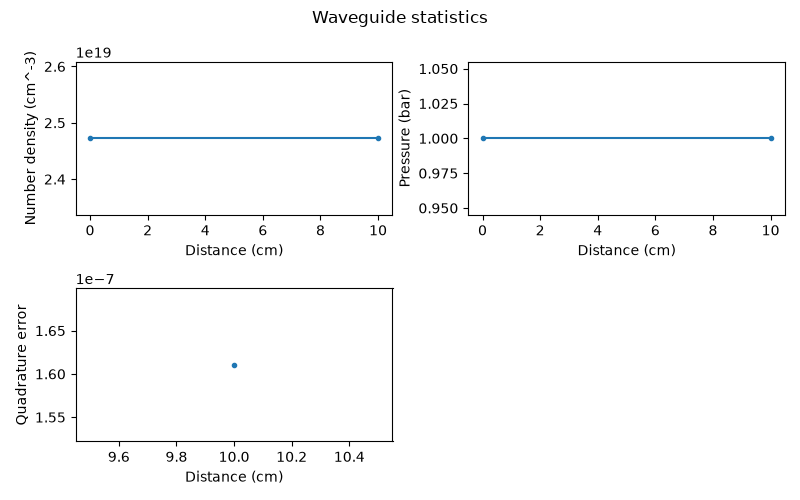
Ten fixed steps of 1 cm. The run’s metadata records that it is per unit width, and the statistics are labelled in uJ/m and W/m. Markers keep the isolated quadrature diagnostic visible when it has only one recorded value.

grid = EnvelopeGrid.from_limits(0.1, 800e-9, (650e-9, 1000e-9), 1.2e-12)
simulation = Simulation.from_waveguide(
    modes.modes,
    0.1,
    "Ar",
    1.0,
    lambda0=800e-9,
    grid=grid,
    absorber=absorber(grid, boundary_length=1e3),
    fwhm=100e-15,
    energy=0.5,
    envelope=True,
    plasma=False,
    raman=False,
    n_save=2,
    dz_max=0.01,
    dz_init=0.01,
    schedule=FixedSchedule(np.full(10, 0.01)),
    backend="numpy_ref",
)
# The driver places a pulse in the first mode; the projected launch is the same
# pulse's spectrum shared among the modes by the Gaussian's overlaps.
pulse = GaussianPulse(wavelength=800e-9, fwhm=100e-15, energy=0.5).build(grid)[0]
launch = np.stack([math.sqrt(share) * pulse for share in shares])
output = simulation.with_input(launch).run(progress="none")
print(output.metadata.transverse_measure)
stats(output, marker="o", markersize=3)

/home/docs/checkouts/solprop/checkouts/24/src/solprop/driver/simulation.py:6500: SolpropWarning: the temporal absorber attenuates a packet walking off by 39.7 fs over 0.1 m by only 0.0085 nepers, below the 6.9 that stops it wrapping around the time window; widen trange, or raise boundary_N above 1.62e+04
  warn_walkoff(grid, span, boundary_length=boundary.in_stage_length)
per_unit_width

[<Figure size 1200x750 with 7 Axes>, <Figure size 800x500 with 3 Axes>]

print(f"ran in {perf_counter() - started:.1f} s on numpy_ref")

ran in 1.6 s on numpy_ref

A hollow planar waveguide, per unit width#

Related reading#