GNLSE propagation: an N = 3 soliton

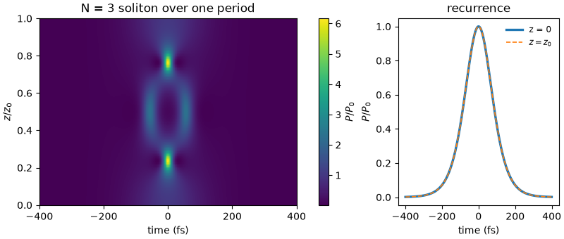
A pulse in anomalous dispersion can balance dispersive spreading against nonlinear self-phase modulation. A fundamental soliton keeps its shape in the ideal cubic nonlinear Schrödinger equation. A higher-order soliton instead changes shape periodically. Here an N = 3 soliton compresses, develops several peaks, and returns to its initial shape after one soliton period.

The GNLSE interface lets us specify dispersion and nonlinear strength directly. For this lesson we retain only second-order dispersion and the instantaneous Kerr response: no loss, Raman response, higher-order dispersion, or self-steepening. These choices give an ideal recurrence problem. They are useful for understanding the balance of effects, but are not a complete model of a particular fibre.

The preceding Resonant dispersive-wave propagation lesson retained the broader physics needed for ultraviolet generation. Removing those perturbations here makes it easier to connect pulse parameters to dynamics. The full equation and available extensions are in Generalised nonlinear Schrödinger propagation.

Choose the pulse and its length scales

The input amplitude is \(A(t)=\sqrt{P_0}\,\mathrm{sech}(t/\tau_0)\). Its intensity FWHM is \(2\operatorname{arcosh}(\sqrt{2})\tau_0\), about \(1.763\tau_0\); width below is \(\tau_0\), not that FWHM. Define the dispersion length \(L_D=\tau_0^2/|\beta_2|\) and nonlinear length \(L_{NL}=1/(\gamma P_0)\). Their ratio fixes the soliton order, \(N^2=L_D/L_{NL}\). Choosing N = 3 therefore sets the peak power rather than leaving it as an independent parameter. The soliton period is \(z_0=\pi L_D/2\).

The example coefficients set useful scales; changing them while holding N fixed rescales distance and power in this ideal equation. The 4 ps time window keeps the pulse tails far from the boundaries, and the wavelength band accommodates the much broader spectrum at compression. See Grids and Fourier conventions.

import time

import matplotlib.pyplot as plt
import numpy as np

from solprop.driver import prop_gnlse
from solprop.fourier import inverse
from solprop.grid import EnvelopeGrid

started = time.perf_counter()

BETA2 = -11.83e-27  # s^2/m, anomalous
GAMMA = 0.11  # 1/(W m)
TAU0 = 100e-15  # s, the natural width of sech(t / tau0)
ORDER = 3

dispersion_length = TAU0**2 / abs(BETA2)
period = np.pi / 2 * dispersion_length
peak_power = ORDER**2 * abs(BETA2) / (GAMMA * TAU0**2)
grid = EnvelopeGrid.from_limits(period, 835e-9, (500e-9, 2e-6), 4e-12)

print(f"dispersion length {dispersion_length:.3f} m, soliton period {period:.3f} m")
print(f"N = {ORDER}: peak power {peak_power:.1f} W")

dispersion length 0.845 m, soliton period 1.328 m
N = 3: peak power 96.8 W

Run one complete period

The controller is asked for a local tolerance of \(10^{-9}\) and the run stores two hundred planes over the period, plus the one at \(z = 0\). Without an output argument the planes are kept in memory; passing a path would stream them to an HDF5 file instead, and that file could be resumed if the run were interrupted.

output = prop_gnlse(
    GAMMA,
    period,
    [0.0, 0.0, BETA2],
    lambda0=835e-9,
    grid=grid,
    width=TAU0,
    peak_power=peak_power,
    pulseshape="sech",
    shock=False,
    rtol=1e-9,
    n_save=201,
    progress="none",
)

z = output["z"]
attempts = output["step_history/counts"].sum()
print(f"{output.n_saved} planes saved, {attempts} steps taken")

201 planes saved, 1128 steps taken

Check the field, including phase

What the handler holds is the stored spectrum at every plane, in the optics convention, and the statistics evaluated there. The recurrence error is the relative distance between the final and the initial spectrum once the expected global phase is removed; in the optics convention that phase is \(+\pi/4\).

stored = output["field"][:, 0, 0]
recurrence = np.linalg.norm(stored[-1] - np.exp(1j * np.pi / 4) * stored[0])
recurrence /= np.linalg.norm(stored[0])
peak_bin = int(np.argmax(np.abs(stored[0])))
phase = float(np.angle(stored[-1][peak_bin] / stored[0][peak_bin]))
print(f"recurrence error after one period: {recurrence:.2e}")
print(f"global phase at the peak bin: {phase:+.5f} rad (expected {np.pi / 4:+.5f})")

recurrence error after one period: 2.65e-09
global phase at the peak bin: +0.78540 rad (expected +0.78540)

Follow compression and recurrence

The evolution over one period. The pulse compresses to a fraction of its width, throws out side lobes, and comes back; the map is symmetric about the half period. The power comes from the same spectra in the internal convention, which is what an inverse transform expects.

power = np.abs(inverse(output.fields("fft")[:, 0, 0], kind="envelope")) ** 2
window = np.abs(grid.t) < 400e-15

fig, (left, right) = plt.subplots(
    1, 2, figsize=(8.0, 3.4), width_ratios=(1.6, 1.0), layout="constrained"
)
mesh = left.pcolormesh(
    grid.t[window] * 1e15,
    z / period,
    power[:, window] / peak_power,
    shading="nearest",
    rasterized=True,
)
left.set_xlabel("time (fs)")
left.set_ylabel("$z / z_0$")
left.set_title(f"N = {ORDER} soliton over one period")
fig.colorbar(mesh, ax=left, label="$P / P_0$")

right.plot(grid.t[window] * 1e15, power[0, window] / peak_power, lw=2.4, label="z = 0")
right.plot(
    grid.t[window] * 1e15,
    power[-1, window] / peak_power,
    lw=1.2,
    ls="--",
    label="$z = z_0$",
)
right.set_xlabel("time (fs)")
right.set_ylabel("$P / P_0$")
right.set_title("recurrence")
legend = right.legend(fontsize="small", frameon=False)

Interpret the recorded statistics

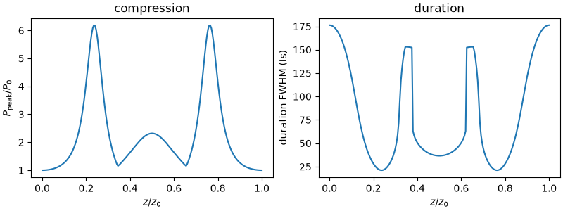
The statistics are recorded at every plane, so the compression is a line rather than a second pass over the fields: the peak power rises about sixfold a quarter of the way in and again three quarters of the way, with the split pulse between them, and the duration follows it down. A single FWHM becomes less informative when the pulse has several peaks, so read it beside the temporal map. Energy should remain constant: measure the largest departure over all saved planes, not just the exit.

fig, axes = plt.subplots(1, 2, figsize=(8.0, 3.0), layout="constrained", sharex=True)
axes[0].plot(z / period, output["stats/peak_power"][:, 0] / peak_power)
axes[0].set_ylabel("$P_\\mathrm{peak} / P_0$")
axes[1].plot(z / period, output["stats/fwhm_t"] * 1e15)
axes[1].set_ylabel("duration FWHM (fs)")
for axis in axes:
    axis.set_xlabel("$z / z_0$")
axes[0].set_title("compression")
axes[1].set_title("duration")

energy = output["stats/energy"][:, 0, 0]
print(f"energy drift over the period: {np.max(np.abs(energy / energy[0] - 1)):.2e}")

energy drift over the period: 5.34e-10

Assumptions and next steps

Recurrence tests the complete field rather than only its energy. Small energy drift is necessary but cannot by itself prove that the pulse shape is accurate. The propagation tolerance controls longitudinal integration, while time-window and spectral-band refinement test different numerical errors. See Numerical methods and accuracy for how to vary these separately.

In real fibres, higher-order dispersion, Raman scattering, loss and self-steepening can break this recurrence. Compare the worked examples of Soliton self-compression and ultraviolet dispersive-wave emission and Raman soliton self-frequency shift in hydrogen before adding those effects to a model. Next, A radial filament in argon leaves the guide for a beam that focuses and ionises in free space.

print(f"{time.perf_counter() - started:.1f} s; backend {output.metadata.backend.name}")

4.2 s; backend numba_cpu