Resonant dispersive-wave propagation

This first complete calculation follows a few-cycle pulse through a helium-filled capillary. Dispersion and nonlinearity reshape the pulse until it self-compresses and emits a resonant dispersive wave (RDW) at a much shorter wavelength. We will choose the model, run it, read spectral and temporal maps, isolate a wavelength band, and inspect modal energies and statistics.

An RDW is radiation whose propagation phase matches that of the nonlinear pulse. It is not simply a harmonic of the carrier. The pump, gas density and guide geometry determine where this phase matching can occur. Here a decreasing gas pressure also changes the dispersion along the guide. For the detailed model see Multimode capillaries: the coherent wall, tapers and gradients; for calculating phase-matching curves see Design tools: soliton numbers and dispersive-wave phase matching.

The case uses a 1 m capillary with 125 μm core radius, filled with helium from 1.2 bar at the entrance towards a vacuum reservoir at the exit. The input is 275 μJ at 800 nm with a 7.5 fs intensity FWHM. We retain two radial HE modes so that the nonlinear response can transfer energy out of the launched fundamental mode. This is a resolved multimode calculation, as introduced in Choosing a spatial description.

Set up and run

prop_capillary takes the core radius, length, gas and pressure first. Lengths, times and energies use SI units; pressure is the user-interface exception, in bar. fwhm is the intensity duration, and the Gaussian pulse energy sets its amplitude. The defaults include waveguide loss, Kerr nonlinearity and plasma.

The field grid resolves the optical carrier, appropriate for this broadband, few-cycle pulse. Its wavelength limits cover the ultraviolet emission as well as the pump; the 200 fs time window leaves room for temporal separation. The guide’s Grids and Fourier conventions chapter explains how to check both choices. n_save controls output sampling, not the adaptive integration step size.

A pressure tuple describes the two reservoirs. The gas-flow model accounts for choking at the evacuated end: the steady flow cannot leave the capillary faster than sound, so the exit sits at its choked pressure, about 7 mbar here, rather than at zero. See Profiles along the fibre for the flow model and its limits. Material-range warnings are silenced for this broad-band lesson: this suppresses a notice, not extrapolation uncertainty. Inspect the material validity ranges when adapting the wavelength band, especially in weak far-ultraviolet wings.

import time
import warnings

import matplotlib.pyplot as plt
import numpy as np

from solprop.driver import prop_capillary
from solprop.exceptions import MaterialRangeWarning
from solprop.plotting import prop_2d, time_1d
from solprop.processing import bandpass, energy, grid_of

started = time.perf_counter()
VUV = (100e-9, 140e-9)

with warnings.catch_warnings():
    warnings.simplefilter("ignore", MaterialRangeWarning)
    run = prop_capillary(
        125e-6,  # core radius, m
        1.0,  # length, m
        "He",
        (1.2, 0.0),  # bar, entrance to exit: a gradient to vacuum
        lambda0=800e-9,
        wavelength_limits=(100e-9, 1.5e-6),
        trange=200e-15,
        fwhm=7.5e-15,
        energy=275e-6,
        modes=2,
        n_save=51,
        progress="none",
    )

print(f"{run['z'].size} planes, {run['field'].shape[1]} modes")
print(f"model: {run.metadata.simulation_kind}; backend: {run.metadata.backend.name}")

51 planes, 2 modes
model: multimode; backend: numba_cpu

Read the unfiltered propagation

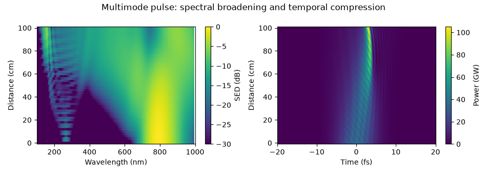
The spectral map shows energy density per unit wavelength in decibels relative to its maximum. The temporal map shows total modal power in the moving time frame. A shift on the time axis means motion relative to that frame, not a negative laboratory arrival time. Follow the compression first, then the emergence and separation of the ultraviolet radiation.

modes="sum" adds modal powers. It does not reconstruct the local transverse intensity: interfering modes require their transverse fields as well. The distinction is developed in Power, energy and intensity.

figures = prop_2d(
    run,
    "wavelength",
    wavelength_range=(100e-9, 1e-6),
    trange=(-20e-15, 20e-15),
    db_min=-30,
    modes="sum",
)
figures[-1].set_size_inches(9.5, 3.4)
figures[-1].suptitle("Multimode pulse: spectral broadening and temporal compression")
figures[-1].tight_layout()

Select the dispersive-wave band

A bandpass selects 100-140 nm from the saved spectrum. Its temporal transform tells us the power and duration of just that spectral component, rather than the whole residual pump. Filtering can broaden or ring a temporal trace, so always state the selected band when quoting a duration or energy.

The conversion efficiency below divides the exit energy in that band by the total input energy. It includes both retained modes and is not a peak spectral density ratio. The window is applied in processing; it does not change the propagation already computed.

grid = grid_of(run)
window = bandpass(grid, VUV)
start = float(np.sum(energy(run, plane=0)))
band = float(np.sum(energy(run, plane=-1, bandpass=window)))
print(f"input {start * 1e6:.1f} μJ, 100-140 nm at the exit {band * 1e9:.2f} nJ")
print(f"conversion efficiency {band / start * 100:.2f} %")

fig, (left, right) = plt.subplots(1, 2, figsize=(9.5, 3.4))
time_1d(run, trange=(-30e-15, 30e-15), modes="sum", ax=left)
left.set_title("Total exit pulse")
time_1d(run, trange=(-30e-15, 30e-15), modes="sum", bandpass=window, ax=right)
right.set_title("Exit pulse filtered to 100-140 nm")
fig.tight_layout()

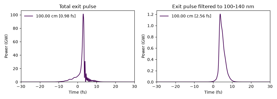
input 275.0 μJ, 100-140 nm at the exit 3688.80 nJ
conversion efficiency 1.34 %

Follow modal energies and plasma

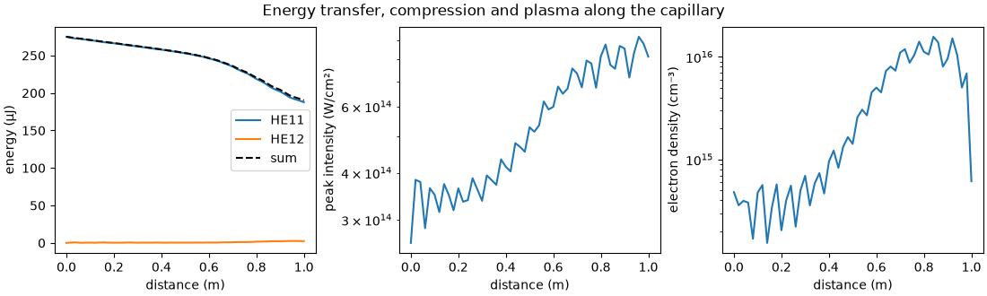
Energy in a higher mode means the transverse field is changing. The modal energy curves also show loss from the retained optical field. Waveguide loss, ionisation and absorbing boundaries can all contribute; the curves alone do not separate them. Peak intensity and electron density help identify when the pulse is strongly compressed and the plasma response is active.

energy(run) processes every saved plane; run["stats/..."] reads statistics collected during propagation. The latter avoids reopening all fields for commonly needed quantities. See Plane statistics for the catalogue and Output: what a run leaves behind for saving and reopening a run.

z = np.asarray(run["z"])
modal_energy = energy(run)
figure, axes = plt.subplots(1, 3, figsize=(11.0, 3.3), layout="constrained")
figure.suptitle("Energy transfer, compression and plasma along the capillary")
for mode in range(modal_energy.shape[1]):
    axes[0].plot(z, modal_energy[:, mode] * 1e6, label=f"HE1{mode + 1}")
axes[0].plot(z, modal_energy.sum(axis=1) * 1e6, "k--", label="sum")
axes[0].set_ylabel("energy (μJ)")
axes[0].legend()
axes[1].semilogy(z, np.asarray(run["stats/peak_intensity"]) * 1e-4)
axes[1].set_ylabel("peak intensity (W/cm²)")
axes[2].semilogy(z, np.asarray(run["stats/electron_density"]) * 1e-6)
axes[2].set_ylabel("electron density (cm⁻³)")
for axis in axes:
    axis.set_xlabel("distance (m)")

Check the approximation before refining the integrator

Two modes provide a useful first picture, not a convergence claim. Add modes and refine transverse quadrature separately from the time window, wavelength band and propagation tolerance. A quadrature diagnostic detects disagreement between transverse integration estimates; it cannot establish that the modal basis itself is large enough. See Radial nodes for expensive responses.

The peak intensity is the on-axis value synthesised from both retained modes. The electron density is read at the quadrature node of largest ionisation, which need not be the axis. Output labels and units matter as much as the numerical value.

alarm = np.asarray(run["stats/quadrature_error"])
finite = alarm[np.isfinite(alarm)]
print(f"largest recorded quadrature diagnostic: {finite.max():.2e}")
print(f"peak on-axis intensity {np.max(run['stats/peak_intensity']) * 1e-4:.3e} W/cm²")
print(
    "peak sampled electron density "
    f"{np.max(run['stats/electron_density']) * 1e-6:.3e} cm⁻³"
)
print(f"{time.perf_counter() - started:.1f} s; backend {run.metadata.backend.name}")

largest recorded quadrature diagnostic: 9.84e-10
peak on-axis intensity 9.189e+14 W/cm²
peak sampled electron density 1.568e+16 cm⁻³
24.2 s; backend numba_cpu

Continue with the idealised GNLSE propagation: an N = 3 soliton to isolate the balance of dispersion and Kerr nonlinearity. For a fuller capillary simulation see Vacuum-ultraviolet dispersive-wave emission in a gas-filled capillary; for changing pressure and geometry see Profiles along the fibre. The high-energy capillary mechanism is discussed experimentally by Travers et al., Nature Photonics 13, 547-554 (2019). This lesson is an illustrative calculation, not a fit to one measurement in that paper.