Two crossing beams in Cartesian free space

Two coherent pulses can overlap, interfere, and then separate without exchanging energy through a nonlinear response. This lesson follows that process in vacuum. Both Gaussian pulses have the same carrier wavelength, duration, polarisation and energy. They enter on opposite sides of the axis at equal and opposite small angles, so their centres cross halfway through the propagation domain.

Unlike the preceding A radial filament in argon, this calculation needs both transverse coordinates. We construct a custom array launch with the existing Simulation API, reconstruct fluence maps, and check the result against linear superposition and elementary beam geometry. There is no nonlinear polarisation, plasma, frequency conversion or four-wave mixing.

Choose geometry and scales

Each beam has a 150 μm waist (1/e² intensity radius), a 70 fs intensity FWHM, and 1 nJ energy at 800 nm. The initial centres are at x = ±0.4 mm. The propagation length is 0.16 m and the carrier angles are approximately ±5 mrad. For centres following straight rays, \(x_\pm(z)=\pm[x_0-z\tan(\theta)]\) and \(z_\mathrm{cross}=x_0/\tan(\theta)\).

At overlap, two plane waves at opposite angles have transverse phase difference \(2k_0 x\sin(\theta)\). Their intensity fringes therefore have spacing \(d=\lambda_0/[2\sin(\theta)]\), about 80 μm. This follows by expanding \(|E_1+E_2|^2\); the cross term is the interference, absent if the beams are mutually incoherent or orthogonally polarised. Finite pulse duration and Gaussian wavefront curvature can reduce contrast or alter local spacing away from overlap.

import time
from dataclasses import replace

import matplotlib.pyplot as plt
import numpy as np
from scipy.optimize import minimize_scalar

from solprop.constants import C
from solprop.driver import Simulation, SimulationSettings
from solprop.grid import EnvelopeGrid, FreeGrid
from solprop.pulses import GaussianPulse
from solprop.spatial import SpatialFlux, SpatialMedium, spatial_energy, spatial_fluence
from solprop.stats import StatsSpec
from solprop.stepper import PIController, RungeKutta

started = time.perf_counter()
LENGTH = 0.16
WAVELENGTH = 800e-9
WAIST = 150e-6
OFFSET = 0.4e-3
ENERGY = 1e-9
VACUUM = SpatialMedium()
angle = np.arctan(2 * OFFSET / LENGTH)
fringe_spacing = WAVELENGTH / (2 * np.sin(angle))
grid = EnvelopeGrid.from_limits(LENGTH, WAVELENGTH, (700e-9, 950e-9), 400e-15)
space = FreeGrid(1.4e-3, 128, 0.8e-3, 48)
temporal = GaussianPulse(wavelength=WAVELENGTH, fwhm=70e-15, energy=ENERGY).build(grid)
print(
    f"angle: {angle * 1e3:.3f} mrad; "
    f"expected fringe spacing: {fringe_spacing * 1e6:.2f} μm"
)
print(f"grid: {space.n_x} x {space.n_y} transverse, {grid.n_t} temporal samples")

angle: 5.000 mrad; expected fringe spacing: 80.00 μm
grid: 128 x 48 transverse, 256 temporal samples

Build a custom array launch

An array passed to Simulation.from_free is a transverse DFT of the temporal spectrum, with shape (n_x*n_y, n_pol, n_omega) in the internal FFT convention. Here there is one polarisation, shared by both pulses. At each temporal frequency we first construct a displaced Gaussian in physical x and y, then apply a tilt, and finally take a two-dimensional spatial FFT. Flattening a (n_y, n_x) array keeps x fastest, as required by FreeGrid.

In the optical convention a beam travelling towards positive x has phase \(\exp(+ik_x x)\). The internal convention is its conjugate, so the code uses a minus sign. Taking \(k_x(\omega)=\omega\sin(\theta)/c\) keeps the angle the same across the pulse’s bandwidth. The reference phase is shared by the beams, and their envelope arrival times agree at the central crossing. See Grids and Fourier conventions and Cartesian free-space propagation before adapting these transforms to measured fields.

spatial_energy measures the physical energy crossing a plane, here in vacuum, with the measure of that plane, a SpatialFlux (Energy and flux in a medium). Normalising each array separately sets equal beam energies; we then add fields, not intensities. For initially overlapping beams, the total energy would also include their interference term.

def launch(spatial_grid, direction):
    """Build one beam; direction +1 starts on the left and travels right."""
    x, y = np.meshgrid(spatial_grid.x, spatial_grid.y)
    profile = np.exp(-((x + direction * OFFSET) ** 2 + y**2) / WAIST**2)
    tilt = np.exp(-1j * direction * x[..., None] * grid.omega * np.sin(angle) / C)
    physical = profile[..., None] * tilt * temporal[0, 0]
    spectrum = np.fft.fft2(physical, axes=(0, 1)).reshape(-1, 1, grid.n_omega)
    flux = SpatialFlux.resolve(grid, spatial_grid, VACUUM)
    return spectrum * np.sqrt(ENERGY / spatial_energy(spectrum, flux))


left = launch(space, +1)
right = launch(space, -1)
settings = SimulationSettings(
    controller=PIController(rtol=1e-7, atol=1e-10),
    integrator=RungeKutta(),
    save_planes=np.linspace(0, LENGTH, 41)[1:],
    dz_init=LENGTH / 40,
    dz_max=LENGTH / 40,
    stats=StatsSpec(names=("energy",)),
    absorber=None,
)
simulation = Simulation.from_free(
    grid,
    space,
    VACUUM,
    [],
    left + right,
    settings=settings,
)
run = simulation.run(progress="none")

Watch overlap and separation

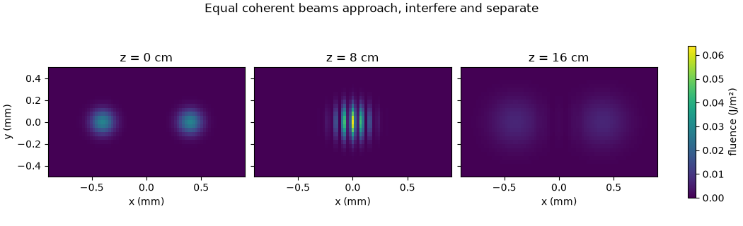
Fluence integrates the axial flux over time and has units J/m². The snapshots show the entrance, the central overlap plane, and the exit on one shared colour scale. Bright and dark fringes at overlap redistribute the local fluence. After the crossing, the beams separate again; their directions have not been changed by a collision. Gaussian diffraction also broadens them during propagation. The x-z map beneath the snapshots takes the y = 0 slice from each saved plane.

z = np.asarray(run["z"])
flux = SpatialFlux.resolve(
    grid, space, VACUUM
)  # one vacuum: one measure at every plane
fluence = np.array(
    [
        spatial_fluence(plane.field, flux).reshape(space.n_y, space.n_x)
        for plane in run.planes()
    ]
)
figure, axes = plt.subplots(
    1, 3, figsize=(10.5, 3.2), layout="constrained", sharey=True
)
figure.suptitle("Equal coherent beams approach, interfere and separate")
for axis, index in zip(axes, (0, 20, 40), strict=True):
    image = axis.pcolormesh(
        space.x * 1e3,
        space.y * 1e3,
        fluence[index],
        shading="auto",
        vmin=0,
        vmax=fluence.max(),
    )
    axis.set_aspect("equal")
    axis.set_xlim(-0.9, 0.9)
    axis.set_ylim(-0.5, 0.5)
    axis.set_xlabel("x (mm)")
    axis.set_title(f"z = {z[index] * 1e2:.0f} cm")
axes[0].set_ylabel("y (mm)")
colourbar = figure.colorbar(image, ax=axes, label="fluence (J/m²)", shrink=0.75)

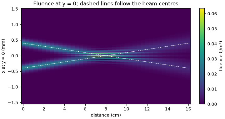
The propagation map makes the approach and subsequent separation easier to follow. The dashed lines mark the centres predicted by the launch angles. Near the crossing, interference creates structure inside the overlapping beams; it does not bend their paths.

figure, axis = plt.subplots(figsize=(7.2, 3.8), layout="constrained")
image = axis.pcolormesh(
    z * 1e2,
    space.x * 1e3,
    fluence[:, space.n_y // 2].T,
    shading="auto",
)
for sign in (-1, 1):
    axis.plot(z * 1e2, sign * (OFFSET - z * np.tan(angle)) * 1e3, "w--", lw=0.8)
axis.set_title("Fluence at y = 0; dashed lines follow the beam centres")
axis.set_xlabel("distance (cm)")
axis.set_ylabel("x at y = 0 (mm)")
colourbar = figure.colorbar(image, ax=axis, label="fluence (J/m²)")

Verify linear superposition and beam motion

Propagate each input separately, saving only the crossing and exit planes for these checks. Adding their complex fields must reproduce the combined run. Adding their fluences instead deliberately omits interference. The centres of the separate beams can still be tracked when the combined pattern has many local maxima. We compare their fluence centroids with the straight-ray estimate.

check_settings = replace(settings, save_planes=np.array([LENGTH / 2, LENGTH]))
individual = []
for initial in (left, right):
    single = Simulation.from_free(
        grid,
        space,
        VACUUM,
        [],
        initial,
        settings=check_settings,
    ).run(progress="none")
    individual.append(single)

superposition_errors = []
centroid_errors = []
individual_fluence = []
for beam, direction in zip(individual, (+1, -1), strict=True):
    maps = np.array(
        [
            spatial_fluence(plane.field, flux).reshape(space.n_y, space.n_x)
            for plane in beam.planes()
        ]
    )
    individual_fluence.append(maps)
    centres = np.sum(maps * space.x[None, None, :], axis=(1, 2)) / maps.sum(axis=(1, 2))
    expected = direction * (-OFFSET + np.asarray(beam["z"]) * np.tan(angle))
    centroid_errors.append(float(np.max(np.abs(centres - expected))))
for combined_index, single_index in ((20, 1), (40, 2)):
    combined = run.fields("fft")[combined_index]
    summed = (
        individual[0].fields("fft")[single_index]
        + individual[1].fields("fft")[single_index]
    )
    superposition_errors.append(
        float(np.linalg.norm(combined - summed) / np.linalg.norm(combined))
    )
energy = np.asarray(run["stats/energy"]).reshape(-1)
energy_error = float(np.max(np.abs(energy / energy[0] - 1)))
collar = (space.window < 1).reshape(space.n_y, space.n_x)
collar_fraction = np.max(fluence[:, collar].sum(axis=1) / fluence.sum(axis=(1, 2)))
print(f"relative field superposition error: {max(superposition_errors):.3e}")
print(f"largest centroid error: {max(centroid_errors) * 1e6:.3e} μm")
print(f"largest relative energy change: {energy_error:.3e}")
print(f"largest energy fraction in the outer collar region: {collar_fraction:.3e}")

relative field superposition error: 5.657e-16
largest centroid error: 5.765e-04 μm
largest relative energy change: 0.000e+00
largest energy fraction in the outer collar region: 3.518e-07

Measure the fringes and refine the spatial grid

At the crossing, divide the interference term by twice the geometric mean of the separate fluences. Near the centre this is approximately a cosine. Fit its spatial period over the illuminated region and compare with the plane-wave prediction. This uses the computed pattern, not a line drawn at the expected spacing.

Double both transverse sample counts at fixed physical size and compare the crossing and exit fluence on the common samples. This checks resolution of the launch tilt and fringes; it does not test a different time window or domain size. This run leaves damping off (absorber=None), so the Fourier domain is periodic. We also report the energy in its outer collar region: negligible boundary illumination is essential if periodic propagation is to approximate open space. Energy conservation alone would not detect light wrapping around. Larger angles, longer propagation, or tighter focusing require fresh boundary, bandwidth and resolution checks; add an absorber when outgoing light reaches the edge. See Absorbing boundaries.

row = space.n_y // 2
a = individual_fluence[0][1, row]
b = individual_fluence[1][1, row]
illuminated = (a > 0.05 * a.max()) & (b > 0.05 * b.max())
x = space.x[illuminated]
contrast = (fluence[20, row, illuminated] - a[illuminated] - b[illuminated]) / (
    2 * np.sqrt(a[illuminated] * b[illuminated])
)
fit = minimize_scalar(
    lambda ratio: np.mean(
        (contrast - np.cos(2 * np.pi * x / (ratio * fringe_spacing))) ** 2
    ),
    bounds=(0.8, 1.2),
    method="bounded",
)
measured_spacing = fit.x * fringe_spacing
fine_space = FreeGrid(space.radius_x, 2 * space.n_x, space.radius_y, 2 * space.n_y)
fine = Simulation.from_free(
    grid,
    fine_space,
    VACUUM,
    [],
    launch(fine_space, +1) + launch(fine_space, -1),
    settings=check_settings,
).run(progress="none")
refinement_errors = []
fine_flux = SpatialFlux.resolve(grid, fine_space, VACUUM)
for fine_plane, coarse_index in zip(list(fine.planes())[1:], (20, 40), strict=True):
    fine_map = spatial_fluence(fine_plane.field, fine_flux).reshape(
        fine_space.n_y, fine_space.n_x
    )
    common = fine_map[::2, ::2]
    refinement_errors.append(
        float(np.linalg.norm(common - fluence[coarse_index]) / np.linalg.norm(common))
    )
print(
    f"fitted fringe spacing: {measured_spacing * 1e6:.3f} μm; "
    f"expected {fringe_spacing * 1e6:.3f} μm"
)
print(
    "largest relative fluence change on spatial refinement: "
    f"{max(refinement_errors):.3e}"
)

# These bounds test physical behaviour with headroom for bandwidth, finite-domain
# tails and discretisation. They are not estimates of experimental uncertainty.
assert max(superposition_errors) < 1e-6
assert max(centroid_errors) < 0.01 * WAIST
assert energy_error < 1e-5
assert collar_fraction < 1e-5
assert abs(measured_spacing / fringe_spacing - 1) < 0.02
assert max(refinement_errors) < 1e-3

figure, axis = plt.subplots(figsize=(7.2, 3.0), layout="constrained")
axis.plot(x * 1e6, contrast, "o", label="computed interference")
x_dense = np.linspace(x.min(), x.max(), 500)
axis.plot(
    x_dense * 1e6,
    np.cos(2 * np.pi * x_dense / fringe_spacing),
    label="plane-wave prediction",
)
axis.set_title("Fringe spacing at the central crossing")
axis.set_xlabel("x at the crossing plane (μm)")
axis.set_ylabel("normalised interference")
axis.legend()
print(
    f"{time.perf_counter() - started:.1f} s including checks; "
    f"backend {run.metadata.backend.name}"
)

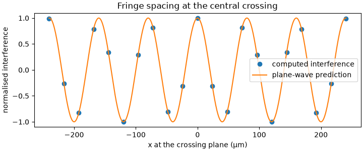
fitted fringe spacing: 80.001 μm; expected 80.001 μm
largest relative fluence change on spatial refinement: 5.960e-16
99.0 s including checks; backend numba_cpu

What to take into another calculation

Spatial arrays carry fields, including phase and polarisation; intensities alone are insufficient to predict interference. This scalar, small-angle example uses identical polarisation and a unidirectional propagation model. Wide angles or tightly focused vector fields require reassessing that model’s assumptions. The vacuum calculation also provides no prediction of nonlinear mixing at the crossing. Start with Cartesian free-space propagation and Polarisation and azimuthal modes before adding that physics.

Continue to Where to go next for task-based routes through the user guide and examples. The focused A Cartesian beam in argon demonstrates adding a material response to a Cartesian beam.