A Cartesian beam in argon#

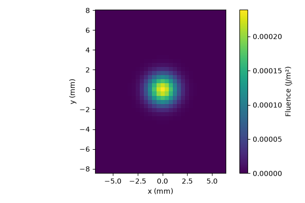
A weak pulsed beam on a Cartesian transverse grid: 800 nm, 30 fs, 1.5 nJ, a 2 mm waist and argon at 4 bar. The energy is the physical energy crossing the entrance plane in the argon (Energy and flux in a medium). The calculation is reduced to a 32 by 40 grid and a 20 mm distance to keep it short.

import matplotlib.pyplot as plt
import numpy as np

from solprop.driver import SimulationSettings, prop_free
from solprop.grid import EnvelopeGrid, FreeGrid
from solprop.nonlinear.responses import KerrResponse
from solprop.physdata import gamma3
from solprop.pulses import GaussianPulse, SpatialPulse
from solprop.spatial import SpatialFlux, SpatialMedium, spatial_fluence
from solprop.stats import StatsSpec
from solprop.stepper import PIController

A matched envelope of the weak field pulse makes the geometry easy to inspect. Each Cartesian component has its own transverse FFT; fields are in V/m. The axes name x first; reshaping flattened columns puts x on the last axis.

length = 0.02
grid = EnvelopeGrid.from_limits(length, 800e-9, (400e-9, 2e-6), 200e-15, thg=False)
space = FreeGrid(6e-3, 32, 7.5e-3, 40)
argon = SpatialMedium("Ar", pressure=4.0)
settings = SimulationSettings(
    controller=PIController(rtol=1e-6, atol=1e-13),
    save_planes=[length],
    dz_init=0.002,
    dz_max=0.002,
    stats=StatsSpec(names=("energy",)),
)
result = prop_free(
    grid,
    space,
    argon,
    [KerrResponse(gamma3("Ar", wavelength=800e-9), thg=False)],
    SpatialPulse(GaussianPulse(wavelength=800e-9, fwhm=30e-15, energy=1.5e-9), 2e-3),
    settings=settings,
)
# The fluence is the time-integrated axial flux, measured in the argon at the exit.
exit_plane = SpatialFlux.resolve(grid, space, argon, z=length)
fluence = spatial_fluence(result.fields("fft")[-1], exit_plane).reshape(
    space.n_y, space.n_x
)
figure, axis = plt.subplots(figsize=(6, 4))
view = axis.pcolormesh(space.x * 1e3, space.y * 1e3, fluence, shading="auto")
axis.set(xlabel="x (mm)", ylabel="y (mm)", aspect="equal")
figure.colorbar(view, ax=axis, label="Fluence (J/m²)")
figure.tight_layout()
print(f"Saved energy: {float(np.asarray(result['stats/energy'])[-1].item()):.6g} J")

Saved energy: 1.5e-09 J

A Cartesian beam in argon#

Related reading#