Comb-to-continuum broadening in hydrogen

A molecular Raman response transfers energy between optical frequencies separated by rotational or vibrational transition frequencies. Repeated scattering can produce a set of Stokes and anti-Stokes sidebands: a Raman frequency comb. As these components broaden and interact, the gaps can fill to form a continuum. We call this comb-to-continuum (CtC) broadening.

Here a 400 fs, 10 uJ pulse at 515 nm propagates through 0.4 m of hydrogen at 40 bar in a capillary of 16 um core radius. The calculation includes the instantaneous Kerr response, rotational and vibrational Raman responses, and photoionisation. Input quantum noise has seed 0. This is one reproducible realisation, not an ensemble: the figure shows how its spectrum develops, but cannot establish shot-to-shot coherence or intensity noise.

We use mode averaging, with the fundamental mode’s effective area and no transverse quadrature. There is no mode conversion, transverse reshaping or spatially resolved plasma. Loss is switched off; the resulting idealised guide does not represent the resonances of a specific antiresonant fibre. The broad computational band also reaches beyond some material fits’ validated ranges. The range warnings are suppressed below; quantitative interpretation of those spectral wings requires checking the material model.

Follow the discrete sidebands in the spectral map and then inspect the four spectral slices. They show the extent of comb formation and merging reached within the stated length; the word continuum is not a claim of a flat or coherent spectrum. Hydrogen’s vibrational shift is approximately 125 THz, so the first vibrational Stokes line from a 515 nm pump is near 655 nm. The calculation uses the full selected Raman model rather than this rounded estimate.

See The Raman response for the line positions, populations and linewidth assumptions, including the shared collisional width of the rotational lines. The Supercontinuum by modulational instability example illustrates ensemble analysis. For an experimental account of comb-to-continuum generation in nitrogen, see Gao et al., From Raman frequency combs to supercontinuum generation in nitrogen-filled hollow-core anti-resonant fiber; its gas and pump conditions differ from this hydrogen calculation.

Set up and run the model

Simulation.from_capillary assembles the material and pulse choices. We then remove its transverse quadrature and request the mode-averaged statistics before translating or running. modes=1 on its own would select a resolved single mode, which is a different nonlinear approximation.

import time
import warnings
from dataclasses import replace

import matplotlib.pyplot as plt

from solprop.driver import Simulation
from solprop.exceptions import MaterialRangeWarning
from solprop.plotting import prop_2d, spec_1d
from solprop.stats import default_spec

started = time.perf_counter()
with warnings.catch_warnings():
    warnings.simplefilter("ignore", MaterialRangeWarning)
    simulation = Simulation.from_capillary(
        16e-6,
        0.4,
        "H2",
        40.0,
        lambda0=515e-9,
        fwhm=400e-15,
        energy=10e-6,
        loss=False,
        plasma=True,
        raman=True,
        trange=4e-12,
        wavelength_limits=(170e-9, 4e-6),
        noise="input",
        seed=0,
        n_save=201,
    )
    simulation.settings = replace(
        simulation.settings,
        quadrature=None,
        components=None,
        stats=default_spec("mode_averaged"),
    )
    assert simulation.translate().flags.mode_averaged
    run = simulation.run(progress="none")
assert run.metadata.simulation_kind == "mode_averaged"
assert run.metadata.quadrature is None
print(f"{run.metadata.simulation_kind}, z = {run['z'][-1]:.2f} m; seed 0")

mode_averaged, z = 0.40 m; seed 0

Spectral and temporal evolution

figures = prop_2d(
    run,
    "wavelength",
    wavelength_range=(200e-9, 2.6e-6),
    trange=(-1e-12, 1e-12),
    db_min=-40,
)
figures[-1].set_size_inches(9.5, 3.6)
figures[-1].suptitle(
    "Hydrogen: spectral comb formation and temporal breakup over 0.4 m"
)
figures[-1].tight_layout()

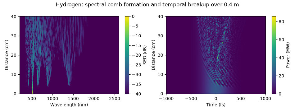
The comb and the continuum

The four positions lie within the 0.4 m calculation. Compare peak locations as well as their broadening: a logarithmic plot can make weak features prominent.

fig, ax = plt.subplots(figsize=(7.0, 4.0))
spec_1d(run, z=[0.05, 0.1, 0.2, 0.4], ax=ax, wavelength_range=(200e-9, 2.6e-6))
ax.set_title("Raman sidebands broaden and overlap along the fibre")
fig.tight_layout()

vibrational_stokes = 1 / (1 / 515e-9 - 4155e2)
print(f"first vibrational Stokes line: {vibrational_stokes * 1e9:.0f} nm")

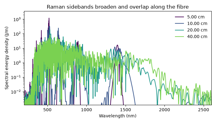
first vibrational Stokes line: 655 nm

The early slices retain conspicuous discrete peaks. By 0.4 m, broadened components overlap across much of the visible and near infrared, with weaker radiation extending farther to the red. The single-shot spectrum remains strongly structured: comb-to-continuum describes the broadening mechanism, not a guarantee of spectral flatness or coherence.

Runtime and next steps

A quantitative noise study needs repeated independent seeds, as in the MI ensemble. For sampling and material checks see Grids and Fourier conventions and Materials: gases, metals and glasses.

print(f"{time.perf_counter() - started:.0f} s; backend {run.metadata.backend.name}")

202 s; backend native