Note
Go to the end to download the full example code.
The vacuum-ultraviolet dispersive wave under a frequency-dependent Kerr response#
The dispersive-wave example runs the canonical
helium case – a 7.5 fs, 275 uJ pulse at 800 nm in 1.5 m of 125 um-radius capillary,
helium falling from 0.8 bar to vacuum, four HE_1m modes, plasma on – with the
default electronic response, which freezes helium’s Kerr coefficient at the 800 nm
carrier and uses it for every quartet the cubic couples. This example repeats that run,
unchanged but for the electronic policy, under the two frequency-dependent responses of
A frequency-dependent electronic response:
"gas-polynomial", optmat’s whole fit of helium’s hyperpolarisability evaluated at the four frequencies of every quartet;"symmetric-kerr", its cheaper symmetric factorisation, exact for self-phase modulation.
The cubic source mixes spectral components of the self-compressing pulse through frequency quartets, so the coefficients that matter belong to quartets with one or more legs between 100 and 150 nm. That is beyond helium’s data: optmat’s fit holds every leg down to its leg bound, 151.9 nm, and beyond it the dispersive responses hold the leg there (the bounded region, a held-coefficient approximation rather than a certified bound on the observable); below helium’s two-photon resonance at a 120.3 nm fundamental, the band edge, no off-resonant model is valid at all, and the same held value is labelled best effort. So this comparison is a sensitivity study – how much the dispersive wave depends on the coefficients of its vacuum-ultraviolet legs, held at the 800 nm value by the carrier policy and at the leg bound’s by the dispersive ones – not a qualified prediction. A resonant helium response, such as the TDSE coupling of TDSE response in a helium capillary, can explore resonant effects, but carries its own atomic-model, finite-window and calibration limitations; it is not an automatically qualified reference.
The second half measures how that sensitivity depends on the mode set, with one, two and four modes, and the last cell separates what the plasma does.
What to look for. The soliton’s own self-phase modulation at 800 nm has the same coefficient under all three policies, and the dispersive wave’s centre moves by only 2-3 nm, as its phase matching to the soliton predicts. Its energy does not: at the exit the 100-150 nm band carries about 30 % more under the dispersive responses than under the carrier one with two or four modes, and about 53 % more with one. The two dispersive evaluators agree to a fraction of a per cent. The pump’s peak power, which oscillates along the second half of the fibre in step under every policy, is a few per cent lower under the dispersive responses; with plasma on, the lower peak ionises less, and about 9 % more energy leaves the fibre.
What is approximate. Everything the dispersive-wave example approximates, and the electronic response of the vacuum-ultraviolet legs, which is the point. A separate refinement study of these runs found that a hundred times tighter step tolerance leaves every band energy and centre unchanged to four digits, and a wider grid (70 nm to 6 um over 600 fs) moves the band energies by less than 1 % and the centres by less than 0.1 nm, so the differences reported here are the models’, not the integrator’s or the grid’s. This page reruns the comparisons at one resolution. Numerical agreement cannot qualify the unknown ultraviolet electronic response.
Start with Resonant dispersive-wave propagation for the workflow. Interpret the comparisons alongside A frequency-dependent electronic response and the separate physical and numerical checks in Assessing numerical accuracy.
The runs#
The run of the dispersive-wave example, with the electronic policy and the mode count as the only arguments. Every run takes the default backend.
import math
import time

import matplotlib.pyplot as plt
import numpy as np

from solprop.constants import C
from solprop.driver import prop_capillary
from solprop.physdata import MaterialSelection
from solprop.processing import (
    bandpass,
    energy,
    get_power,
    get_spectral_density,
    grid_of,
)
from solprop.processing.time import moment

POLICIES = ("carrier-kerr", "symmetric-kerr", "gas-polynomial")
COLOURS = {policy: f"C{index}" for index, policy in enumerate(POLICIES)}
VUV = (100e-9, 150e-9)
"""The band the dispersive wave is counted in, m."""

started = time.perf_counter()


def m2_run(policy, modes=4, plasma=None):
    """Propagate the helium dispersive-wave case under one electronic policy."""
    return prop_capillary(
        125e-6,  # core radius, m
        1.5,  # length, m
        "He",
        (0.8, 0.0),  # bar, entrance to exit
        lambda0=800e-9,
        fwhm=7.5e-15,
        energy=275e-6,
        modes=modes,
        trange=400e-15,
        wavelength_limits=(90e-9, 4e-6),
        plasma=plasma,
        n_save=151,
        materials=MaterialSelection(electronic=policy),
        progress="none",
    )


def band_along(run):
    """Return the dispersive wave's energy at every saved plane, J."""
    window = bandpass(grid_of(run), VUV)
    planes = np.asarray(run["z"]).size
    return np.array(
        [float(np.sum(energy(run, plane=i, bandpass=window))) for i in range(planes)]
    )


def centre_wavelength(run):
    """Return the energy-weighted centre of the band at the exit, m."""
    band = (2 * math.pi * C / VUV[1], 2 * math.pi * C / VUV[0])
    frequency, density = get_spectral_density(
        run, "omega", plane=-1, modes="sum", spec_range=band
    )
    return 2 * math.pi * C / moment(frequency, density)


runs = {policy: m2_run(policy) for policy in POLICIES}
z = np.asarray(runs["carrier-kerr"]["z"])
The regions#
A dispersive run records, for each gas, where its active band falls: supported (every leg within helium’s data), bounded (beyond the leg bound, inside the band edge) and best effort (beyond the band edge). Here the band runs to 82 nm, so all three occur, and the dispersive wave’s band straddles the last two.
supported     151.9 -  8000.0 nm
bounded       120.3 -   151.9 nm
best_effort    81.8 -   120.3 nm
The dispersive wave and the pump#
The energy of the 100-150 nm band along the fibre, the peak power of the pump, and the exit spectrum below 400 nm with the bounded (light) and best-effort (dark) bands shaded; four modes, summed.
fig, (left, middle, right) = plt.subplots(
    1, 3, figsize=(13.0, 3.8), layout="constrained"
)
summary = {}
for policy, run in runs.items():
    along = band_along(run)
    _, power = get_power(run, modes="sum", oversampling=4)
    peak = power.max(axis=1)
    summary[policy] = (
        along[-1],
        centre_wavelength(run),
        peak.max(),
        float(np.sum(energy(run, plane=-1))),
    )
    left.plot(z, 1e6 * along, lw=1.6, color=COLOURS[policy], label=policy)
    middle.plot(z, 1e-9 * peak, lw=1.4, color=COLOURS[policy], label=policy)
    wavelength, density = get_spectral_density(
        run, "wavelength", plane=-1, modes="sum", spec_range=(85e-9, 400e-9)
    )
    right.semilogy(
        1e9 * wavelength,
        density / density.max(),
        lw=1.0,
        color=COLOURS[policy],
        label=policy,
    )
for name, shade in (("bounded", "0.88"), ("best_effort", "0.72")):
    low, high = regions[name]
    right.axvspan(
        1e9 * low, 1e9 * high, color=shade, lw=0, zorder=0, label=name.replace("_", " ")
    )
left.set_xlabel("z (m)")
left.set_ylabel("100-150 nm energy (uJ)")
left.legend(frameon=False)
middle.set_xlabel("z (m)")
middle.set_ylabel("peak power (GW)")
middle.set_xlim(0.9, 1.5)
right.set_xlim(85, 400)
right.set_ylim(1e-5, 2.0)
right.set_xlabel("wavelength (nm)")
right.set_ylabel("exit spectrum (normalised)")
right.legend(frameon=False, fontsize="small", ncols=2)

reference = summary["gas-polynomial"]
for policy, (band, centre, peak, total) in summary.items():
    print(
        f"{policy:15s} 100-150 nm {1e6 * band:6.2f} uJ "
        f"({100 * (band / reference[0] - 1):+5.1f} % of the polynomial's), "
        f"centre {1e9 * centre:6.2f} nm; largest peak power {1e-9 * peak:4.0f} GW; "
        f"{1e6 * total:.1f} uJ at the exit"
    )
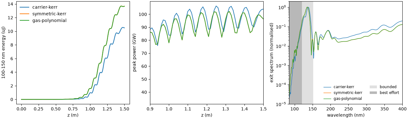
carrier-kerr    100-150 nm  10.49 uJ (-23.2 % of the polynomial's), centre 134.51 nm; largest peak power  106 GW; 142.1 uJ at the exit
symmetric-kerr  100-150 nm  13.68 uJ ( +0.1 % of the polynomial's), centre 132.14 nm; largest peak power  102 GW; 155.3 uJ at the exit
gas-polynomial  100-150 nm  13.66 uJ ( +0.0 % of the polynomial's), centre 132.19 nm; largest peak power  102 GW; 155.0 uJ at the exit
The pump’s peak power oscillates along the second half of the fibre with a period of about 7 cm, in step under every policy, and is a few per cent lower under the dispersive responses. The dispersive wave’s centre is set by phase matching to the soliton’s nonlinear wavenumber, which comes from self-phase modulation at the carrier, identical under every policy; it moves by 2-3 nm. Its energy grows by about 30 %: every quartet that makes a vacuum-ultraviolet photon has its VUV leg held at helium’s leg bound, 151.9 nm, by the dispersive responses, and the whole quartet at the 800 nm Kerr value by the carrier one. The symmetric factorisation, whose error grows with the spread of a quartet’s four frequencies, is within a fraction of a per cent of the polynomial even here.
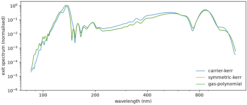
The whole exit spectrum, on a logarithmic wavelength axis: away from the vacuum ultraviolet the three are hard to tell apart.
fig, ax = plt.subplots(figsize=(8.0, 3.4), layout="constrained")
for policy, run in runs.items():
    wavelength, density = get_spectral_density(
        run, "wavelength", plane=-1, modes="sum", spec_range=(85e-9, 1.3e-6)
    )
    ax.semilogy(
        1e9 * wavelength,
        density / density.max(),
        lw=1.0,
        color=COLOURS[policy],
        label=policy,
    )
ax.set_xscale("log")
ax.set_xticks([100, 200, 400, 800], labels=["100", "200", "400", "800"])
ax.set_ylim(1e-6, 2.0)
ax.set_xlabel("wavelength (nm)")
ax.set_ylabel("exit spectrum (normalised)")
_ = ax.legend(frameon=False)
The sensitivity by mode count#
The same three policies with one and two modes. The mode set changes the soliton’s dynamics, and with them how much the exit band depends on the vacuum-ultraviolet coefficients.
by_modes = {4: {policy: summary[policy][:2] for policy in POLICIES}}
del runs  # the four-mode fields are no longer needed
for modes in (2, 1):
    by_modes[modes] = {}
    for policy in POLICIES:
        run = m2_run(policy, modes=modes)
        by_modes[modes][policy] = (band_along(run)[-1], centre_wavelength(run))

print("modes  carrier   symmetric  polynomial (uJ)   carrier vs polynomial")
for modes in (1, 2, 4):
    bands = [1e6 * by_modes[modes][policy][0] for policy in POLICIES]
    change = 100 * (bands[0] / bands[2] - 1)
    print(
        f"{modes:5d}  {bands[0]:7.2f}  {bands[1]:9.2f}  {bands[2]:10.2f}       "
        f"{change:+6.1f} %"
    )

fig, ax = plt.subplots(figsize=(5.0, 3.4), layout="constrained")
counts = (1, 2, 4)
for offset, policy in zip((-0.25, 0.0, 0.25), POLICIES, strict=True):
    ax.bar(
        np.arange(3) + offset,
        [1e6 * by_modes[m][policy][0] for m in counts],
        width=0.25,
        color=COLOURS[policy],
        label=policy,
    )
ax.set_xticks(np.arange(3), labels=[f"{m} mode{'s' * (m > 1)}" for m in counts])
ax.set_ylabel("100-150 nm energy at the exit (uJ)")
_ = ax.legend(frameon=False, fontsize="small")
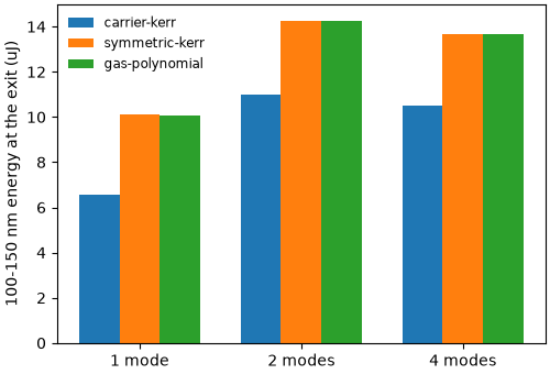
modes  carrier   symmetric  polynomial (uJ)   carrier vs polynomial
    1     6.58      10.10       10.06        -34.6 %
    2    10.98      14.26       14.24        -22.9 %
    4    10.49      13.68       13.66        -23.2 %
With two and four modes the dispersive responses give the band about 30 % more energy than the carrier policy; with one, about 55 % more. The two-mode reduced case of the tutorial (one metre, 1.2 bar, a narrower grid) differs by about 9 %. The sensitivity is a property of the case and its mode set, not one number: report it with them.
Where the plasma comes in#
With plasma on, the dispersive runs’ lower peak power went with less energy lost (above). The same two policies without plasma, four modes:
for policy in ("carrier-kerr", "gas-polynomial"):
    run = m2_run(policy, plasma=False)
    _, power = get_power(run, modes="sum", oversampling=4)
    peak = power.max(axis=1)
    print(
        f"{policy:15s} no plasma: largest peak power {1e-9 * peak.max():4.0f} GW; "
        f"100-150 nm {1e6 * band_along(run)[-1]:.2f} uJ; "
        f"{1e6 * float(np.sum(energy(run, plane=-1))):.1f} uJ at the exit"
    )
carrier-kerr    no plasma: largest peak power  128 GW; 100-150 nm 12.29 uJ; 220.3 uJ at the exit
gas-polynomial  no plasma: largest peak power  118 GW; 100-150 nm 14.75 uJ; 220.3 uJ at the exit
Without plasma the dispersive response’s peak power is lower again, by 8 %, its dispersive wave a fifth stronger, and the energy leaving the fibre the same. So the lower peak is the electronic response’s own; with plasma on, it ionises less, and the pump keeps about 13 uJ more to the exit.
Runtime and reproducibility#
print(f"{time.perf_counter() - started:.0f} s; backend {run.metadata.backend.name}")
53 s; backend native
Total running time of the script: (0 minutes 52.868 seconds)