A frequency-dependent electronic response#

The Kerr response multiplies the cube of the field by one number per gas: its electronic third-order susceptibility frozen at the run’s carrier. That number is not a property of the gas alone. A gas’s hyperpolarisability rises towards the ultraviolet — argon’s Kerr coefficient at 267 nm is twice its value at 800 nm, xenon’s at 400 nm nearly twice its value at 2 µm — and for a quartet of different frequencies it depends on all four. A run whose spectrum spans an octave or more, or which mixes widely separated colours, therefore uses a coefficient that is right for some of its processes and wrong for others.

This page describes the two dispersive electronic policies of SEP 6, which evaluate optmat’s whole fit of a gas’s hyperpolarisability at the absolute frequencies of every quartet the cubic couples, in one broadband polarisation. It is for readers who want to know which polarisation such a run computes, what each of the two evaluators approximates and what it costs, what happens where the field leaves the gas’s data, and how to read what a run recorded. The tutorial runs both of SEP 6’s demonstration cases under all three policies.

`MaterialSelection.electronic`	Response	What it evaluates
`"recommended"`, `"carrier-kerr"` (the default)	`KerrResponse`	the Kerr coefficient at the carrier, one number per gas and run (materials)
`"gas-polynomial"`	`DispersiveKerrResponse`, evaluator `"polynomial"`	optmat’s gas dispersion polynomial, exactly, at every quartet
`"symmetric-kerr"`	`DispersiveKerrResponse`, evaluator `"symmetric"`	a symmetric factorisation of the polynomial’s Kerr diagonal (a mixture’s: of the mixture’s own)

Both dispersive policies are opt-in; the carrier policy stays the default. They run on numpy_ref, numba_cpu and the native backend’s CPU build on every route: the capillary and radial routes, Cartesian and line free space, the planar route and a general modal guide’s gas regions. The native backend’s device builds are qualified for them on one AMD Instinct generation (HIP) and one NVIDIA Hopper device (CUDA). A run is never moved to another backend or another response without being told.

One susceptibility, all mixing processes#

In the optics Fourier convention (conventions, §2) the third-order polarisation of a real scalar field is one double integral over the input frequencies,

\[ \widetilde P^{(3)}(\omega_o)=\frac{\varepsilon_0}{(2\pi)^2} \iint\chi^{(3)}(-\omega_o;\omega_1,\omega_2,\omega_3)\, \widetilde E(\omega_1)\widetilde E(\omega_2)\widetilde E(\omega_3) \,\mathrm d\omega_1\,\mathrm d\omega_2, \qquad \omega_3=\omega_o-\omega_1-\omega_2 . \]

Self- and cross-phase modulation, four-wave mixing and third-harmonic generation are not separate terms: they are slices of the same integral, \((\omega,\omega,-\omega)\to \omega\), \((\omega_r,\omega_p,-\omega_p)\to\omega_r\), \((\omega_p,\omega_p,-\omega_i)\to2\omega_p-\omega_i\) and \((\omega,\omega,\omega)\to3\omega\). With a constant \(\chi^{(3)}\) the integral collapses to \(\varepsilon_0\chi^{(3)}E(t)^3\), which is why the constant cubic needs no bookkeeping of processes. A dispersive susceptibility must keep that property: one polarisation, every quartet weighted by its own four frequencies, no process named during propagation.

For a gas of number density \(N\) with Taylor-convention second hyperpolarisability \(\gamma_T\), \(\chi^{(3)} = N\gamma_T/(6\varepsilon_0)\), and solprop’s per-particle coefficient is \(\gamma^{(3)} = \gamma_T/(6\varepsilon_0)\) in m⁵/V² (materials). optmat fits \(\gamma_T\) over a quartet of signed vacuum wavenumbers \(\nu_j=\omega_j/2\pi c\), the output counted negative so that the four sum to zero, with the dispersion expansion of Bishop and De Kee, J. Chem. Phys. 104, 9876 (1996), doi:10.1063/1.471752 (their Eqs. 22 and 67, written there additively in atomic units), put relative to the static value in Shelton’s form:

\[ \gamma_T=\gamma_0\,[1+A S_2+B S_2^2+B' S_4],\qquad S_2=\textstyle\sum_j\nu_j^2,\quad S_4=\sum_j\nu_j^4 . \]

Its Kerr diagonal, \((\nu,\nu,-\nu)\to\nu\), is \(\gamma_K(\nu)/\gamma_0 = 1+4A\nu^2+(16B+4B')\nu^4\); the carrier policy uses \(\gamma_K\) at the carrier for every quartet. optmat’s records carry \(A\) in units of \(10^{-10}\) cm² and \(B\), \(B'\) in \(10^{-20}\) cm⁴, which solprop takes to m² and m⁴ (DispersiveKerrModel).

Why a coefficient of the output frequency is wrong#

The tempting shortcut multiplies the constant cubic’s spectrum by the Kerr coefficient of each output frequency, \(\varepsilon_0\chi_K(\omega)\mathcal F[E^3]\). It is right for monochromatic self-phase modulation and wrong for everything else. It gives every quartet that lands on a frequency the degenerate coefficient of that frequency, whatever its inputs were: the argon quartet \(400+400-800\to266.7\) nm gets argon’s Kerr value at 266.7 nm, 50 % above the polynomial’s value for that quartet, where the carrier’s value at 400 nm is only 4 % below it (table below). It also breaks the exchange symmetry of a lossless quartet — the coefficient changes when a different member is called the output — so the response does net work on the field, which a transparent medium cannot. solprop does not offer it.

The two evaluators#

Both evaluate the cubic as a sum of products of spectrally filtered fields, transformed on the run’s oversampled fine grid; neither builds a table over frequency triplets. The filters are real, even functions of absolute frequency, so the same response is computed on a field grid and on an envelope grid at any carrier.

The polynomial ("gas-polynomial"). With \(D\) the spectral multiplier \(d(\omega)=(\omega/2\pi c)^2\), expanding \(S_2\) and \(S_4\) over the four legs and grouping the output factors gives (SEP 6, §4.5)

\[ \frac{6\widetilde P}{N\gamma_0} =[1+Ad+(B+B')d^2]\,\mathcal F[E^3] +[3A+6Bd]\,\mathcal F[E^2\,DE] +\mathcal F\big[3(B+B')\,E^2D^2E+6B\,E(DE)^2\big]. \]

This is exact evaluation of the fit on the resolved grid: no approximation beyond the fit itself. It costs three inverse transforms (of \(E\), \(DE\), \(D^2E\)) and three forward transforms of products where the constant cubic needs one of each.

The symmetric factorisation ("symmetric-kerr"). One real, even multiplier \(g(\nu)=[\gamma_K(\nu)/\gamma_0]^{1/4}\) is applied to every leg:

\[ \chi^{(3)}_{\rm sym}=\chi_0\,g(\nu_o)g(\nu_1)g(\nu_2)g(\nu_3), \qquad P_{\rm sym}=\varepsilon_0\chi_0\,G\big[(GE)^3\big], \]

with \(G\) the filter \(g\): filter the field, cube it, filter the polarisation. It is exact on the Kerr diagonal and agrees with the polynomial through second order in the frequencies for every quartet; its leading error is \((B-A^2/2)\sum_{j<k}(\nu_j^2-\nu_k^2)^2\), which grows with the spread of the quartet’s four frequencies. Over random quartets between 400 nm and 2 µm the median error is 0.006 % for helium and 0.05 % for argon and the largest 0.1 % and 0.9 %; xenon, the most dispersive gas, reaches 3 % (SEP 6, §4.7). For a scalar field with no other response it needs no transform beyond the constant cubic’s, only two spectral multiplications, since the filters can act on the spectra the cubic already transforms.

Matching every degenerate value does not determine the general susceptibility: the factorisation is a separability assumption, not a consequence of the data, and the polynomial is the reference it is measured against.

Cost. The symmetric evaluator adds spectral multiplications to transforms already needed for the cubic response. The polynomial requires derivative fields and additional transforms; mixtures can share them where their leg bounds agree. Whole-run cost also depends on the adaptive trajectory, so stage cost alone does not predict the runtime. Use the backend and performance guide for execution choices. The measured stage-time ratios against the constant cubic, with their conditions, are in the benchmarks.

The temporal collar. A run’s temporal collar \(w(t)\), which keeps the polarisation off the edges of the time window, multiplies each product in time before its output multipliers and \(\Pi_+\): \(G[w\,(GE)^3]\), and likewise for every term of the polynomial. The constant cubic’s collar multiplies its polarisation, and with no output multiplier the two orders coincide. For the dispersive evaluators the difference depends on the filtered fields and products near the collar. Check it by enlarging the window while retaining resolution. The earlier comparison found a difference of a few parts in \(10^3\) for a pulse at nine tenths of the half-window. A statement of equivalence for a well-contained pulse is conditional on the filtered field also remaining clear of the collar.

Lossless response. With no active temporal collar or boundary term, both kernels are real and symmetric in their four legs. The continuum response then does no net work on a real field, \(\int(\partial_tE)\,P\,\mathrm dt=0\), exactly as the constant cubic. Discrete evaluation requires adequate sampling; an occupied collar changes this identity. Energy conservation in a propagation therefore requires checking absorbers, representation error and integration error together. The test suite compares both evaluators with an explicit input-triplet sum at \(10^{-14}\) and checks the lossless identity.

The harmonic sector: `thg`#

The constant cubic’s thg=False keeps “the fundamental band” by a narrowband rule (one cubic, four forms). The dispersive responses use a rule that holds at any bandwidth instead. Writing the real fields through their analytic signals, each product of three fields is a sum over quartets whose four signed legs have three, two or one positive members:

`thg`	Sector	Quartets kept
`True` (the field-grid default)	full	all: self- and cross-phase, four-wave mixing, the third harmonic and its inverse
`False` (the envelope-grid default)	number-conserving	two positive and two negative legs, with \(\Pi_+\), the projection onto positive absolute frequency

The number-conserving sector is \(\mathrm{Re}\{\tfrac34\Pi_+[|u|^2u]\}\) for a field of analytic signal \(u\), with the filters of the evaluator applied to each leg. It keeps no harmonic quartet, so it conserves photon number as well as energy. With the dispersion removed, and for any band narrower than an octave, it is exactly the constant cubic’s thg=False rule; beyond an octave the constant rule, which lacks \(\Pi_+\), does a little net work and the dispersive sector does none. The general modal route’s kerr_form maps the same way — "real" to the full sector, "analytic" to the conserving one — for a region that declares its gas fill (GasKerr); a region with a constant MaterialKerr keeps it under every policy (general modal propagation).

On an envelope grid the full sector carries two harmonic groups, \(\mathrm e^{+2\mathrm i\omega_0t}\) as the constant cubic’s harmonic does, and \(\mathrm e^{-2\mathrm i\omega_0t}\), the one-into-three exchange that reaches positive frequencies only for a field wider than an octave. An envelope grid built for harmonics (EnvelopeGrid.from_limits(..., thg=True)) holds both for a field inside its active band: a super-octave field agrees with a four-times finer evaluation to \(10^{-13}\). Like the constant cubic’s harmonic, both groups can still wrap around the grid when the field itself reaches the edges of the active band — when its collars hold content — so keep the band wide enough that they stay empty.

Beyond the gas’s data: bounded, never refused#

A run’s field routinely extends far beyond any gas’s data: a helium RDW run reaches below 80 nm. The carrier policy runs there with a constant extrapolated from the carrier. The rule for the dispersive policies is never to be less sound than that, and never to refuse a run for the frequencies its field occupies (SEP 6, §4.10). It rests on three facts optmat publishes in the support record of each hyperpolarisability model:

The legs of the data. The four signed legs of a quartet sum to zero, so no leg of a quartet within the fitted frequency sums \(S_{2,\max}\) exceeds \(\nu_c=\sqrt{3S_{2,\max}/4}\), the leg bound.
The resonances. A single leg reaches the lowest dipole-coupled level \(E_1\) and a pair of legs the lowest two-photon level \(E_2\); a field stays clear of both while it occupies wavelengths longer than the band edge, \(\min(E_1, E_2/2)\). A vector run, with two polarisation components, takes the band edge for any polarisation, which is 1–3 nm longer for Ne, Ar, Kr, Xe and CO.
Monotonicity. Every fit rises with each \(\nu_j^2\), inside its data and beyond. No theorem requires the physical \(\gamma\) to do the same, but every curated calculation rises towards the first resonance, and faster than the fit.

solprop holds every leg of both evaluators at the leg bound, \(\nu_j\to\min(|\nu_j|,\nu_c)\): the polynomial’s multiplier becomes \(\min(d(\omega),\nu_c^2)\) and the symmetric filter is evaluated at \(\min(|\nu|,\nu_c)\). Both stay real, even and the same on every leg, so the lossless identity and the cost are unchanged, and no quartet within the fitted sums moves. The run’s active band (half its lowest frequency to 1.1 times its highest) is classified at translation, per gas, into three regions:

Region	Where	What the evaluators give	How to read it
supported	legs within \(\nu_c\), inside the band edge	the fit itself	exact within the fit; beyond \(S_{2,\max}\), the polynomial’s own extrapolation
bounded	beyond \(\nu_c\), inside the band edge	each such leg held at \(\nu_c\)	a bounded estimate: clamping can underestimate a rising off-resonant response, but optmat does not certify a bound on the true coefficient or the observable
best effort	beyond the band edge, or beyond \(\nu_c\) for a gas whose edge is undefined	the same bounded evaluation	the off-resonant fit is unqualified there; the response is held at the data edge rather than continuing its \(\nu^4\) growth through a resonance

A run whose band reaches the bounded or best-effort region logs that once, at INFO, naming the gas and the band; nothing is refused and nothing warns per step. The leg bounds and band edges are optmat’s, read from its support record, never written into solprop; at optmat 0.8.0 (unchanged since 0.4.0), for one linear polarisation:

Gas	Leg bound (nm)	Band edge (nm)
He	151.9	120.3
Ne, Ar	215.9	133.5, 189.4
Kr, Xe	230.1	216.7, 256.0
H₂, D₂	215.9, 224.7	201.7, 201.1
N₂, O₂	215.9, 224.7	290.1, 304.6
CO	231.5	308.9
CO₂, CH₄, SF₆, N₂O, O₃	230.1, 224.7, 215.9, 383.4, 401.0	undefined: no curated two-photon limit, so best effort beyond the leg bound

Air has no fit of its own; each of its populations carries its own, and O₂ makes air best effort below about 305 nm. CO₂, CO and O₃ have optmat fits but are not yet built-in species.

Pump dynamics and emission in one response#

A resonant dispersive wave in the vacuum ultraviolet is emitted through four-wave mixing: three components of the self-compressing soliton produce a VUV photon. Neither dispersive evaluator gives a band one coefficient, so modelling that emission costs nothing at the pump. In the helium RDW case of SEP 6:

the soliton’s self-phase modulation at 800 nm keeps \(\gamma_K(800\,\mathrm{nm})\), exactly the carrier value, and its broadened wings, down to about 250 nm at maximum compression, lie inside helium’s data and are evaluated exactly;
a generating quartet such as \(250+250-1500\to136.4\) nm takes a coefficient set by all four of its legs, 1.41 times the 800 nm value under the leg bound (1.49 unbounded), where the carrier policy is about 30 % low; in the symmetric model the single VUV leg enters only as a fourth root;
the largest coefficients belong to quartets with two or more VUV legs — the cross-phase modulation of the dispersive wave by the pump, its own self-phase modulation — and they scale with the weak dispersive-wave field, so they hardly act back on the pump.

The dispersive wave’s wavelength is set by phase matching to the soliton’s nonlinear wavenumber, which comes from the exactly evaluated self-phase modulation, so it moves little between the policies; its energy, and its evolution after emission, are what change. In the full-size case (the worked example) the 100–150 nm band at the exit carries about 30 % more energy under both dispersive policies than under the carrier one with two or four modes, and about 53 % more with one, and its centre moves by 2–3 nm; in the tutorial’s shorter two-mode case, about 9 % and a nanometre. Below helium’s 120.3 nm band edge that is a sensitivity to the treatment of the VUV legs, not a qualified prediction: a resonant response, such as the helium TDSE response, can investigate those effects, subject to its own atomic-model and finite-window limitations. It is not an automatically qualified reference there. That response owns helium’s whole electronic response, so a dispersive policy is refused beside it for the same gas.

The demonstration cases in numbers#

The coefficients each policy assigns to the quartets of SEP 6’s two demonstration cases, from optmat’s fits; errors are signed relative to the polynomial, and \(S_2/S_{2,\max}\) above one is beyond the fitted sums. The leg-bounded column is what the runs use, as a fraction of the unbounded polynomial.

Quartet (nm)	Gas	\(\gamma_{\rm poly}/\gamma_K(800)\)	Carrier error (%)	Symmetric (%)	Output-only (%)	\(S_2/S_{2,\max}\)	Bounded / polynomial
400 + 400 − 800 → 266.7	Ar	1.345	−4.25 at 400; −25.65 at 800	+0.556	+50.00	0.98	1
SPM of 266.7	Ar	2.018	−36.17 at 400; −50.44 at 800	0	0	1.97	1
XPM of 266.7 by 400	Ar	1.612	−20.13 at 400; −37.98 at 800	−0.025	+25.13	1.42	1
250 + 250 − 1500 → 136.4	He	1.485	−32.68 at 800	−0.012	+88.95	1.49	0.949
SPM of 120	He	3.679	−72.82 at 800	0	0	4.81	0.628
SPM of 80	He	11.27	−91.13 at 800	0	0	10.81	0.205

In argon every leg stays above the 215.9 nm leg bound, so the bounded evaluation is the polynomial itself, and every frequency is inside the 189.4 nm band edge. The generating quartet’s carrier error at the 400 nm pump is small; the signal’s cross-phase modulation by the pump is 20 % stronger than the carrier says, and in the tutorial that, not the generating coefficient, is what moves the conversion: the dispersive runs convert faster at first and saturate earlier, about 30 % below the carrier run at the exit of half a metre. In helium the VUV quartets are bounded and, below 120.3 nm, best effort; the bound takes self-phase modulation at 80 nm from the raw polynomial’s 11.3 times the 800 nm value to 2.31 times.

The map below shows the symmetric factorisation’s error over degenerate-pump four-wave mixing, \(2\omega_p-\omega_i\to\omega_s\), for argon and helium, with the boundaries of the fitted sums and of the regions. The contours at 0.1, 1 and 5 % are descriptive levels, not acceptance thresholds.

import matplotlib.pyplot as plt
import numpy as np
from matplotlib.lines import Line2D

from solprop.physdata.nonlinear_data import OptmatKerr

pump, idler = np.meshgrid(np.linspace(250e-9, 1000e-9, 241),
                          np.geomspace(520e-9, 4e-6, 241))
with np.errstate(divide="ignore"):
    signal = 1.0 / (2.0 / pump - 1.0 / idler)
kept = idler > pump

fig, axes = plt.subplots(1, 2, figsize=(9.5, 3.9), layout="constrained",
                         sharey=True)
for ax, gas in zip(axes, ("Ar", "He")):
    model = OptmatKerr(gas).dispersive_model()
    legs = np.stack([1 / signal, 1 / pump, 1 / pump, 1 / idler], axis=-1)
    polynomial = model.gamma3(legs)
    weights = model.kerr_ratio(np.minimum(legs**2, model.leg_bound**2))
    symmetric = model.gamma3_static * np.prod(weights**0.25, axis=-1)
    error = np.where(kept, 100 * np.abs(symmetric / polynomial - 1), np.nan)
    x, y = 1e9 * pump, 1e6 * idler
    filled = ax.contourf(x, y, np.log10(np.clip(error, 1e-4, 10)),
                         levels=np.linspace(-4, 1, 21), cmap="Blues")
    lines = ax.contour(x, y, error, levels=[0.1, 1.0, 5.0], colors="0.15",
                       linewidths=0.8)
    ax.clabel(lines, fmt=lambda value: f"{value:g} %", fontsize="small")
    sums = np.sum(legs**2, axis=-1) / (4 * model.leg_bound**2 / 3)
    ax.contour(x, y, np.where(kept, sums, np.nan), levels=[1.0], colors="C4",
               linestyles="--", linewidths=1.3)
    ax.contour(x, y, np.where(kept, 1 / signal, np.nan),
               levels=[model.leg_bound, model.band_edge(vector=False)],
               colors=["C1", "C3"], linestyles=[":", "-."], linewidths=1.3)
    ax.set_title(f"{gas}: $2\\omega_p - \\omega_i$")
    ax.set_xlabel("pump wavelength (nm)")
    ax.set_yscale("log")
    ax.set_yticks([0.6, 1, 2, 3, 4], ["0.6", "1", "2", "3", "4"])
    ax.minorticks_off()
axes[0].plot([400], [0.8], marker="*", color="C1", markersize=11,
             markeredgecolor="k", linestyle="none")
axes[0].set_ylabel(r"idler wavelength ($\mu$m)")
axes[1].legend(
    [Line2D([], [], color="C4", ls="--"), Line2D([], [], color="C1", ls=":"),
     Line2D([], [], color="C3", ls="-.")],
    ["fitted sums", "signal at the leg bound", "signal at the band edge"],
    loc="upper right", fontsize="small", framealpha=0.9)
fig.colorbar(filled, ax=axes, label="log$_{10}$ symmetric error (%)")

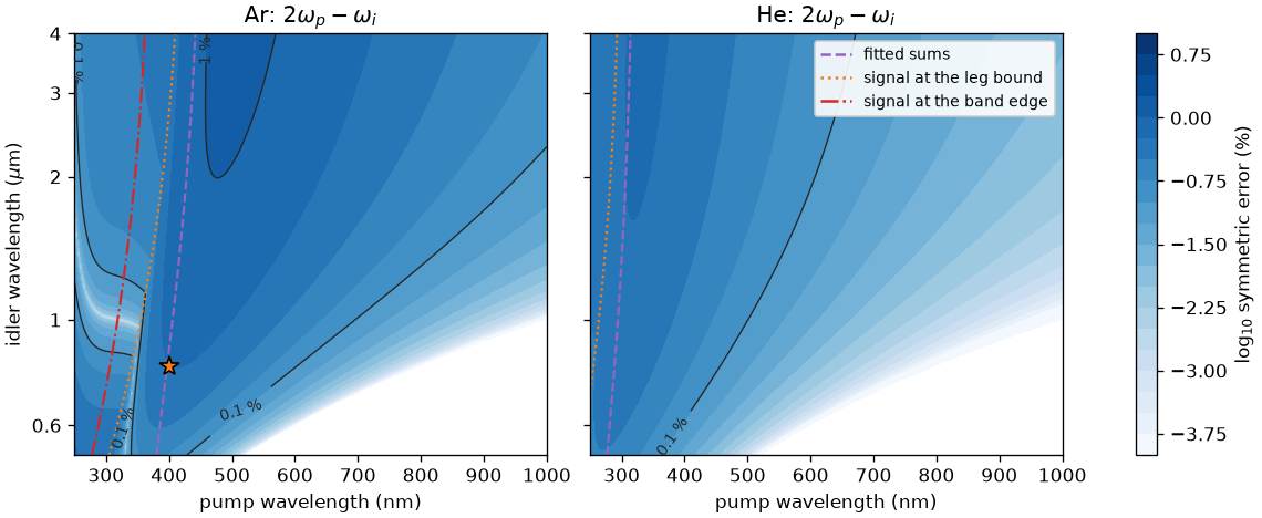
Contour maps of symmetric-factorisation error versus pump and idler wavelengths for argon and helium, with material-support boundaries marked. — The symmetric factorisation against the polynomial for degenerate-pump four-wave mixing, both under the leg bound, as a function of the pump and idler wavelengths. Left of the dashed purple line the quartet is beyond the fitted frequency sums; left of the dotted line the signal’s leg is held at the leg bound (bounded); left of the dash-dotted line the signal is beyond the band edge (best effort). The star is the argon DUV quartet of the tutorial. Where the bound holds a leg the two evaluators move together, and the error falls again.#

Mixtures and vectors#

The polynomial of a mixture is the exact per-species sum. Each population of a mixture is its own channel, with its own multipliers, leg bound and density path: \(P=\sum_s\varepsilon_0\gamma_{0,s}N_s\,\mathrm{cubic}_s(E)\). Species whose leg bounds are equal share their filtered fields \(DE\) and \(D^2E\), and their coefficient tables add, density-weighted, \(\sum_sN_s\gamma_{0,s}(1,A_s,B_s,B'_s)\) — an exact rewriting, which numba_cpu takes for every such mixture, so that its transforms grow with the number of distinct leg bounds rather than of species. Krypton and xenon share one, as do argon, H₂ and SF₆, neon and N₂, and D₂, O₂ and CH₄; air’s three species have three.

The symmetric evaluator of a mixture factorises the mixture’s own curve. Different filters do not reduce to one summed coefficient as the constant cubic’s do, so the exact per-species symmetric sum, \(\sum_s\varepsilon_0\gamma_{3,s}N_s\, G_s[w(G_sE)^3]\), would cost one product per species. The symmetric evaluator instead takes one filter from the mixture’s own Kerr diagonal, \(\gamma_{K,\rm mix}(\nu)=\sum_sN_s\gamma_{K,s}(\tilde\nu_s)\), each species’ leg bounded at its own \(\nu_c\), and factorises it exactly as it factorises one gas:

\[ P=\varepsilon_0\Big(\sum_sN_s\gamma_{3,s}\Big)\,G_{\rm mix}\big[w\,(G_{\rm mix}E)^3\big], \qquad g_{\rm mix}(\omega)=\left[\frac{\sum_sN_s\gamma_{3,s}\hat K_s(\omega)} {\sum_sN_s\gamma_{3,s}}\right]^{1/4}, \]

with \(\hat K_s=\gamma_{K,s}(\tilde\nu_s)/\gamma_{3,s}=g_s^4\) each species’ own bounded Kerr diagonal. On the Kerr diagonal the four legs give \(\varepsilon_0\sum_sN_s\gamma_{3,s}\,g_{\rm mix}^4=\varepsilon_0\gamma_{K,\rm mix}\), the mixture’s degenerate coefficient, exactly; the reference, the mixture’s static coefficient, cancels as it does for one gas. A mixture costs what one gas costs. The filter depends on the composition, not on the total density: where the populations have different density paths along z — independent partial pressures, say — it is rebuilt from their densities at every stage; a fill of constant composition builds it once. One species is its own operator exactly.

Off the diagonal the mixture’s filter is an approximation of the exact per-species symmetric sum, which remains the test reference. By the survey of SEP 6 §4.7 (quartets on 400–2000 nm) it departs from that sum by at most 0.016 % for helium and argon and 0.045 % for air (medians 0.0005 %), fifty times less than the symmetric factorisation’s own departure from the polynomial, 0.9 % and 1.3 %: as an approximation of the polynomial the mixture’s filter is as good as the exact sum. In a 3 cm, 150 µJ capillary run the exit field’s nonlinear change departs from the polynomial’s by 0.29 % (helium and argon) and 0.36 % (air), against 0.27 % and 0.29 % for the exact sum and 5–6 % for the carrier policy (SEP 6).

A supplied species, which carries no optmat model, is refused under a dispersive policy by name rather than given a borrowed curve; air resolves through its populations.

Vectors use the isotropic Kleinman tensor. Two polarisation components contract through \(T_{ijkl}=(\delta_{ij}\delta_{kl}+\delta_{ik}\delta_{jl}+\delta_{il}\delta_{jk})/3\), so that three filtered fields give \(\tfrac13[(X\cdot Y)Z+(X\cdot Z)Y+(Y\cdot Z)X]\), which is \((E\cdot E)E\) when they coincide. This is a named approximation: Kleinman’s ratio \(\chi_{xxyy}=\chi_{xxxx}/3\) is held at every frequency. optmat’s \(\gamma\) is the mean over parallel linear polarisations, and the distinct dispersion of the tensor’s components is not represented. The run records it as "isotropic-kleinman".

When the carrier is enough, and which evaluator to choose#

What the demonstration cases measured#

Both of SEP 6’s demonstration cases were run at full size, under all three policies on the default backend, in the worked examples the dispersive wave under a frequency-dependent response and deep-ultraviolet four-wave mixing in argon. Each difference below is the carrier policy’s against the polynomial’s, and the symmetric evaluator’s against the polynomial’s. Values are rounded from the recorded example output.

Case	Observable	Carrier	Symmetric
Helium dispersive wave, four modes	100–150 nm energy at the exit	−23 %	+0.1 %
	the same, two modes; one mode	−23 %; −35 %	+0.1 %; +0.4 %
	its centre wavelength	+2.3 nm	−0.05 nm
	the pump’s largest peak power; the energy leaving the fibre	+4 %; −8 %	0 %; +0.2 %
	the same without plasma	+8 %; 0 %	not run
Argon four-wave mixing, 1 m	the best pressure	+10 mbar (+5 %)	same
	the largest signal energy at each policy’s own best pressure	+1.7 %	+0.4 %
	the signal at the carrier’s best pressure; at the linear phase matching	+11 %; +20 %	0 %; 0 %

Two kinds of result appear. In argon, the quartets the case drives have every leg within the gas’s leg bound and inside its band edge, so the dispersive responses are exact relative to optmat’s fit and the carrier column is the carrier approximation’s error. It sits in the phases: the signal’s cross-phase modulation by the pump is a quarter stronger than the carrier coefficient says, which moves the phase matching, while the best attainable conversion hardly changes. In helium the dispersive wave’s quartets reach past the leg bound and the band edge, so the carrier column is a sensitivity of the observable to the coefficients of its vacuum-ultraviolet legs, which no off-resonant model fixes; it depends on the mode set, by a factor of 1.5 here.

By observable#

Self-phase modulation and the pump near the carrier. The carrier coefficient is exact for self-phase modulation at the carrier under every policy. What it misses is the variation of the Kerr diagonal over the occupied band: \(\gamma_K\) rises by 12 % from 2 µm to 400 nm in helium, 37 % in argon and 87 % in xenon (SEP 6, §4.7). For a band where that variation is small against what a result needs, the carrier policy is adequate. In the helium case the pump’s peak power, which oscillates along the fibre in step under every policy, is 4–8 % lower under the dispersive responses; with plasma on the lower peak ionises less, and about 9 % more energy leaves the fibre.
A band generated far from the carrier — a dispersive wave, a four-wave-mixing signal, ultraviolet light from a near-infrared pump. Its energy depends on quartets with legs far from the carrier, and on its cross- and self-phase modulation, whose coefficients differ from the carrier’s by tens of per cent (the demonstration-case table above). Use a dispersive policy; where the band is bounded or best effort, run the carrier policy beside it and report the spread.
A phase-matched wavelength — a dispersive wave’s centre, a signal’s wavelength. Set by linear phase matching to a nonlinear wavenumber that the carrier mostly gets right, it moves by a few nanometres.
An operating point — the pressure or energy that maximises a conversion. The nonlinear phases move it; the carrier policy can misplace it by several per cent and misjudge the yield at a given setting by tens of per cent while agreeing on the best yield.

A coefficient error of one per cent need not mean a one per cent error in a phase-matched conversion. Where in doubt, run the observable under the carrier policy and under a dispersive one: the difference is the carrier approximation’s cost for that observable.

Which evaluator#

"symmetric-kerr" is often close in cost to the carrier response; see the two evaluators for the work each requires. In both demonstration cases it stays close to the polynomial, within half a per cent on the dispersive wave and about a per cent across the argon scan: it is the one to use for production runs and scans. Its error is largest for quartets of widely spread frequencies in the most dispersive gases — xenon, krypton, O₂, CH₄ and SF₆ reach 1.7–3.2 % on random quartets between 400 nm and 2 µm (SEP 6, §4.7) — so check it against the polynomial there.

"gas-polynomial" is exact relative to optmat’s fit and is the reference the symmetric evaluator is measured against. Its extra transforms usually make it more expensive, particularly for a mixture with distinct leg bounds, such as air, whose species cannot share the same derivative fields. Use it to check the symmetric evaluator, for a result that must be exact relative to the fit, and for mixtures whose species share a leg bound (krypton and xenon cost what one gas costs).

The symmetric error against the fit’s own uncertainty#

The fits are not exact either. For the quartets of §4.7 of SEP 6 (random frequencies between 400 nm and 2 µm inside each fit’s data), the table sets the symmetric evaluator’s departure from the polynomial beside the one-sigma statistical uncertainty of the same quartet’s dispersion, \(\gamma(q)/\gamma_0\), propagated from the covariance of optmat’s \(A\), \(B\) and \(B'\) (scaled by the reduced \(\chi^2\) where that exceeds one). Both columns are median / maximum in per cent; the last is the fraction of quartets whose symmetric error exceeds that uncertainty (SEP 6’s fit-uncertainty study).

Gas	Symmetric error	Fit’s one sigma	Error above sigma
He	0.006 / 0.124	0.015 / 0.109	0.26
Ne	0.007 / 0.153	0.141 / 0.274	0.00
Ar	0.053 / 0.913	0.162 / 0.366	0.21
Kr	0.115 / 1.714	1.066 / 3.197	0.00
Xe	0.260 / 3.212	0.481 / 2.682	0.32
H₂, D₂	0.047 / 0.718	0.063 / 0.499	0.42
N₂	0.047 / 0.837	0.209 / 0.437	0.10
O₂	0.183 / 2.908	0.500 / 1.415	0.23
CH₄	0.133 / 1.831	0.404 / 1.353	0.17
SF₆	0.105 / 2.141	0.491 / 1.019	0.11
N₂O	0.048 / 0.656	2.265 / 5.109	0.00

The symmetric evaluator’s typical error is below the fit’s statistical uncertainty of the dispersion in every gas; its largest errors, at the most widely spread quartets, exceed it in a tenth to two fifths of the quartets for most gases. The uncertainty is measured here relative to the static \(\gamma_0\); relative to the pump’s own Kerr value the correlated part cancels and it is several times smaller, so the comparison depends on what a result is normalised to. A covariance is not a bound on the expansion’s truncation, on borrowed priors (N₂O’s dispersion is CO₂’s) or on the systematic errors optmat’s accuracy page lists.

What the regions mean for a result#

The run’s manifest records, per gas, the part of its active band in each region; the region table above says what the evaluators give there. For a result:

for supported quartets, the polynomial evaluates the declared fit and the symmetric policy approximates it. Accuracy of an observable also depends on the fit’s physical validity, the propagation model and numerical convergence;
a result depending on bounded legs is a model estimate. The coefficient may underestimate a rising off-resonant response, but this does not bound the generated energy or conversion efficiency;
one that depends on best-effort legs uses an unqualified continuation: report it as a sensitivity, with the carrier result beside it, never as a correction of the carrier result. A resonant response requires its own atomic-model and numerical qualification before it can provide a reference.

The label is per frequency of the active band, not per quartet the field drives: a run whose band reaches the bounded region is labelled so even where the field there is negligible. Look at where the observable’s band and its generating quartets lie.

Backends#

Both evaluators run on numpy_ref, numba_cpu and the native backend’s CPU build on every route but the GNLSE, agreeing with numpy_ref to a few times machine epsilon, and on the native backend’s device builds, qualified on one AMD Instinct generation and one NVIDIA Hopper device. backend="auto" therefore runs them on the native backend where it is installed, as the carrier policy runs; nothing falls back.

Reading what a run recorded#

A run’s material manifest records the law it used. Its policies["electronic_response"] names the law, the evaluator, the sector, the tensor approximation and the leg-bound rule, with each population’s support-record digest and regions; for a symmetric mixture, mixture_filters names each mixture filter, its rule, the general modal region it acts in (None elsewhere) and the composition it is built from — each population’s label and the SHA-256 identity of its density path. Its electronic entries hold, per population, the model’s name and digest, the leg bound and both band edges in m⁻¹, the regions as wavelength intervals in m, and, in a symmetric mixture, the mixture filter it belongs to (filter). The policies enter the resume key, so a run never resumes under another law, another model, another band or another composition. Inspecting a run before propagating it costs only its translation:

from solprop.driver import Simulation
from solprop.physdata import MaterialSelection

simulation = Simulation.from_capillary(
    50e-6,
    0.5,
    "Ar",
    0.2,
    lambda0=400e-9,
    wavelength_limits=(210e-9, 2e-6),
    trange=250e-15,
    fwhm=30e-15,
    energy=10e-6,
    backend="numba_cpu",
    materials=MaterialSelection(electronic="gas-polynomial"),
)
manifest = simulation.material_manifest()
manifest.policies["electronic_response"]["law"]  # 'gas-polynomial'
(entry,) = manifest.electronic
(
    entry["evaluator"],
    entry["sector"],
    entry["tensor"],
)  # polynomial, full, isotropic-kleinman
entry["regions"]["bounded"]  # [1.909e-07, 2.159e-07]: 190.9 to 215.9 nm
entry["regions"]["best_effort"]  # None: the band stays inside argon's band edge

After a run the same manifest is output.metadata.materials, and the tutorial shades the regions on a spectrum from it.

Limitations#

No resonant response. Both evaluators are off-resonant expansions. In the best-effort region they give a held constant, not physics; nonlinear absorption and the imaginary part of the susceptibility near a resonance are not modelled, and the real kernel is not a causal material law there.
No tensor dispersion. The isotropic Kleinman tensor holds one ratio at every frequency (above).
Gases only. Fused silica keeps its carrier-evaluated cubic: its degenerate \(n_2\) curve does not determine its nondegenerate response, and no curated nondegenerate silica data exist to factorise. A GNLSE run’s fitted \(\gamma\) is a constant coefficient, and refuses a dispersive policy by name; on the general modal route only a region declaring its gas fill takes the dispersive response.
The fits’ own uncertainties remain. Being exact relative to a fit does not remove its absolute-scale and dispersion uncertainty, the vibrational contributions some molecular fits retain, or N₂O’s dispersion borrowed from CO₂ (optmat’s records say which).
The region check is per frequency of the active band. It does not identify which quartets a field actually drives; a band that reaches the bounded region is labelled so even if the field there is negligible.
Backends. numpy_ref, numba_cpu and the native backend’s CPU build on every route but the GNLSE (single-mode, multimode, radial, Cartesian and line free space, planar, general modal); the native backend’s device builds on one AMD Instinct generation (HIP) and one NVIDIA Hopper device (CUDA).

This page documents the functionality proposed and implemented by SEP 6.