Nonlinear responses#
A response says how a medium answers a field: the nonlinear polarisation P(t) it
produces at a point of the cross-section, given the field there and the local density.
Every nonlinear effect solprop propagates — self-phase modulation, third-harmonic
generation, photoionisation, Raman scattering — enters through one.
Use Kerr to describe instantaneous electronic refraction and frequency mixing, Raman for a delayed molecular or glass response, and plasma for ionisation and free-electron currents. The effects can act together: a pulse can compress, excite molecular motion and ionise the medium in one calculation.
This chapter introduces their different time behaviour, then derives the Kerr polarisation and its projection into propagation. Continue to Raman, ionisation rates, carrier-resolved plasma or envelope plasma for the corresponding models. A frequency-dependent electronic response is available when one carrier-frequency Kerr coefficient is insufficient. Where solprop’s choices differ from Luna.jl’s, the differences are listed in Noteworthy differences from Luna.
Three different kinds of memory#
An instantaneous Kerr index change follows the local intensity. A delayed Raman response can keep oscillating after the excitation. Ionisation accumulates an electron population, so its refractive contribution can persist after the pulse in a model without recombination. Their different time dependence helps explain why they produce different frequency shifts and pulse shapes.
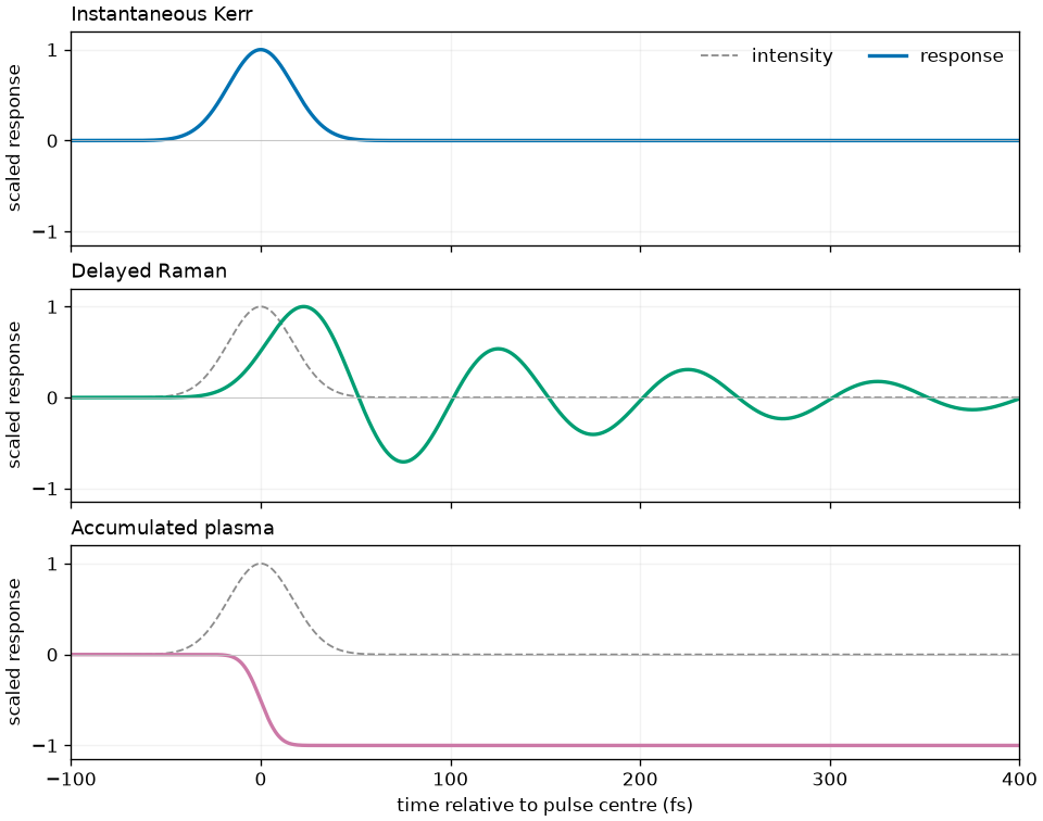
Illustrative response shapes, not a propagation or a fit to a material. The grey dashed line is a Gaussian intensity pulse. The Raman curve is its convolution with an arbitrary damped oscillator; the plasma curve is a negative accumulated intensity-to-the-fifth-power proxy. Each response is scaled independently. The chosen times merely separate the three behaviours; use the material models for quantitative predictions.#
Choosing and combining responses#
Configure the physical processes before choosing numerical resolution. Gas-filled
waveguide constructors accept kerr, raman and plasma switches or explicit
response choices. Free-space calculations take an explicit response sequence:
naming a gas supplies its linear properties, but does not enable every nonlinearity.
The radial filament lesson
shows Kerr and envelope plasma together.
A response acts on the local electric field in V/m. In a resolved calculation, solprop reconstructs that field across the cross-section and projects the resulting source back onto the propagated channels. A mode-averaged calculation instead uses an effective-area model. Choosing only one resolved mode does not make those two calculations identical.
Not every response runs on every grid. Kerr, dispersive Kerr and
RamanResponse accept both; carrier-resolved plasma
and SilicaTensorResponse need a field grid, and
envelope plasma an envelope grid. The
response trait table lists each
response’s grids, polarisation forms and z profiles.
chi3 is the susceptibility per unit of the density argument. A gas passes the
per-particle hyperpolarisability \(\gamma_3\) together with its number density, and a fixed
medium passes \(\chi^{(3)}\) with a density of one. This is the convention the kernel
contract’s density profile assumes.
Check whether the quoted nonlinearity includes Raman. A medium
whose Raman strength is stated as a share \(f_R\) of its total nonlinearity has a Kerr
coefficient that was already reduced by \((1 - f_R)\) when the response is constructed —
solprop.nonlinear.gnlse.kerr_susceptibility() does exactly that for a fibre GNLSE —
and a molecular gas’s Raman response is absolute, built from its own molecular constants,
with the full electronic \(\chi^{(3)}\) beside it. Solprop does not additionally apply
\((1 - f_R)\) itself: doing so would either double the reduction or invent one, and with
Raman switched off it would simply discard part of the nonlinearity.
The Kerr response#
The instantaneous third-order polarisation of an isotropic medium is \(P_i = \varepsilon_0 \chi^{(3)} \rho\, E_i |E|^2\) in the scalar case, and the whole of the subtlety is in what “\(E\)” means on each grid.
One cubic, four forms#
Write the field through its analytic signal. On a field grid the state is the real \(E = \mathrm{Re}\,E_a\); on an envelope grid it is \(A = E_a\mathrm{e}^{-\mathrm{i}\omega_0 t}\), so that \(E = \mathrm{Re}(A\mathrm{e}^{\mathrm{i}\omega_0 t})\) (the algorithms, §5; internal FFT convention, conventions §2). Cubing the real field with \(\theta = \omega_0 t\),
With thg=True, the real-field cubic contains both terms. With thg=False,
solprop instead evaluates the analytic-signal fundamental approximation shown in
the table below. On an envelope grid, retaining the harmonic requires spectral
room for it and an explicit \(\mathrm{e}^{2\mathrm{i}\omega_0 t}\) to sit at the right
offset from the carrier. Writing \(P = \mathrm{Re}(P_\text{env}\mathrm{e}^{\mathrm{i}\theta})\),
which is the envelope form of Genty et al., Opt. Express 15, 5382 (2007). The \(\mathrm{e}^{+2\mathrm{i}\omega_0 t}\) sign follows from \(E_a = A\mathrm{e}^{+\mathrm{i}\omega_0 t}\) in the internal FFT convention. The sign is tied to the envelope convention, so it is derived here rather than transcribed from the literature. The factor carries no \(z\) dependence, which holds only because \(t\) is a pure retarded time: the frame must keep the carrier phase whole, removing neither \(\beta_0\) nor the constant \(-\beta_1\omega_0\) that a delay measured from the carrier would remove (which terms the frame removes). A regression test compares the third harmonic of a short hydrogen capillary on the two grids and against the closed-form weak-conversion estimate.
The four cases solprop.nonlinear.responses.KerrResponse.evaluate() implements are
therefore
grid |
|
polarisation |
|---|---|---|
field |
|
\(\varepsilon_0\chi^{(3)}\rho\,E^3\) |
field |
|
\(\tfrac34\varepsilon_0\chi^{(3)}\rho\,\lvert E_a\rvert^2 E\) |
envelope |
|
\(\tfrac34\varepsilon_0\chi^{(3)}\rho\,\lvert A\rvert^2 A\) |
envelope |
|
\(\tfrac14\varepsilon_0\chi^{(3)}\rho\,(3\lvert A\rvert^2 + \mathrm{e}^{2\mathrm{i}\omega_0 t}A^2)A\) |
The second and third rows describe the same fundamental-band approximation in real-field and envelope form. Their narrowband agreement is checked in the test suite. For broadband fields whose mixing bands overlap, excluding the nominal third-harmonic frequency range is not by itself a proof of equivalence to the complete real-field cubic.
The vector form falls out of the same algebra#
For two transverse components the fundamental-band content of the cubic is, per component,
with \(a\) the analytic signal or the envelope. Expanded for \(p = x\) this is \(\tfrac34\big[(|a_x|^2 + \tfrac23|a_y|^2)a_x + \tfrac13 a_x^{*}a_y^2\big]\) — the familiar isotropic split into a cross-phase term and a coherent-coupling term — and for one component it collapses to \(\tfrac34|a|^2a\). Writing it as the two sums rather than as the expansion is not a trick: the same two sums also give the harmonic term, \(\tfrac14\big(\sum_q a_q^2\big)a_p\,\mathrm{e}^{2\mathrm{i}\omega_0 t}\), and the same expression serves one component and two.
On a field grid with thg=False the vector form is the same construction applied to the
analytic signal, taking the real part.
A coefficient that depends on frequency#
Everything above multiplies the cubic by one \(\chi^{(3)}\), which for a built-in gas is
its Kerr coefficient at the run’s carrier (materials).
A gas’s electronic response is in fact a function of all four frequencies of each
quartet, and rises towards the ultraviolet. The dispersive electronic policies of
SEP 6,
MaterialSelection(electronic="gas-polynomial") and "symmetric-kerr", replace the
constant by optmat’s whole fit, evaluated at the absolute frequencies of every quartet
in the same single broadband polarisation:
DispersiveKerrResponse, a convolution response
on both grids. Its two evaluators, its harmonic sectors (where thg selects the full
cubic or a number-conserving sector that holds at any bandwidth), the bound it places on
the frequencies beyond a gas’s data and the regions a run records are on
their own page.
From polarisation to propagation#
The nonlinear term of the propagation equation is the transformed polarisation times
which is solprop.nonlinear.normalisation.uppe_prefactor(). Three remarks.
Only the real part of the index appears. That is a modelling choice: the coupling of Kolesik and Moloney’s equation (PRE 70, 036604 (2004), Eq. 28) carries the complex longitudinal wavenumber. solprop keeps the loss once, in the linear operator; the effect of dropping \(\mathrm{Im}\,n_\text{eff}\) here is of relative order \(\mathrm{Im}\,n_\text{eff}/\mathrm{Re}\,n_\text{eff}\). Ferrando et al. (PRE 71, 016601 (2005)) make the same choice in their modal forward–backward equations, to keep the transverse operator self-adjoint.
The \(\omega\) in the numerator is the optical shock term. Self-steepening is not a
separate operator applied in the time domain but the frequency dependence of this
prefactor, so shock=False freezes the numerator at the carrier and changes nothing
else. The index in the denominator is part of the projection and stays frequency
dependent.
The prefactor is zero outside the active band, not one. Leaving the out-of-band bins untouched would leave raw, unnormalised polarisation in the rest of the array; a per-step re-windowing of the state would hide that from the answer, but every Runge-Kutta stage and every error estimate would see it.
Several modes at once#
With a mode set the polarisation is evaluated at quadrature nodes of the cross-section and projected back (capillary modes), which for the Kerr term on a field grid is exactly the cube of a sum:
The \(\varepsilon_0c/2\) that makes the basis orthonormal is folded into the projection matrix, which is why the prefactor above appears here as \(-\mathrm{i}\omega/4n_\text{eff}\). The effective index is each mode’s own, so the multimode and mode-averaged routes use the same normalisation.
Two things follow that are worth having in mind.
The modes are multiplied at the same time sample. Nothing in the sum realigns them, so they have to be written in the same time origin — which is why a mode set shares one co-moving frame (the linear operator) rather than one per mode. The group-delay walk-off between them is then physics the equation carries, not a coordinate choice.
The coupling is testable in closed form. With a weak pump in the fundamental, a weak seed in a second mode, a constant fill and a length short enough for first order, the mode-2 amplitude follows the mode-1 one by
a dimensionless ratio in which \(\chi^{(3)}\), the shock term, the third harmonic and the transform normalisation all cancel: only the overlap ratio and the phase mismatch are left. For two \(\mathrm{HE}_{1m}\) modes of a 125 µm capillary at 800 nm, \(\Delta\beta = 100.68\) rad/m, so 2 cm gives 2.014 rad, a mismatch factor of modulus \(0.8394\) and a ratio of \(0.4017\) at the carrier. A propagation measures \(0.3995\) averaged over a 30 fs pulse’s band, against \(0.3987\) for the same average of the closed form: the difference is the pump’s own dispersion, which this expression drops. Keep it — integrate the first-order solution along \(z\) rather than assuming the pump frozen — and the propagation agrees with it to better than \(10^{-5}\); the test suite asserts this.
Watts and volts per metre#
Mode-averaged propagation carries an amplitude in \(\sqrt{\mathrm{W}}\) and a response
needs V/m. The conversion is the effective area
(solprop.nonlinear.normalisation.sqrtw_to_vm()), applied to the internal,
vacuum-normalised amplitude \(a\):
The middle expression is the vacuum-admittance intensity, which is what this factor defines. It is not the true power per effective area: the power is \(P=|b|^2=w|a|^2\) with \(w=\operatorname{Re}n_{\rm eff}\) (power and intensity), so \(P/A_\text{eff}\) exceeds it by \(w\) — 0.56 % at 20 bar argon or 40 bar hydrogen, 0.03 % at 1 bar argon. The rate models are unaffected by the distinction, because they take the physical electric field \(E_a\) in V/m, the left-hand side above, and not an intensity (see ionisation).
solprop.nonlinear.normalisation.mode_average_prefactor() is the two composed: the
whole mode-averaged normalisation, written in one place. The transform normalisation —
the crop and pad factors of fourier — is not included: it belongs to the grid, and the
translation layer folds it in.
A worked example#
Two hundred kilowatts in a helium-filled capillary, and the polarisation it drives.
import matplotlib.pyplot as plt
import numpy as np

from solprop.grid import FieldGrid
from solprop.nonlinear.normalisation import sqrtw_to_vm
from solprop.nonlinear.responses import KerrResponse
from solprop.physdata import Gas, chi3

grid = FieldGrid.from_limits(1.0, 800e-9, (200e-9, 3e-6), 60e-15)
t = grid.t_fine
aeff = 0.48 * np.pi * (125e-6) ** 2   # a Marcatili HE11 mode of a 125 um core

sigma = 10e-15 / (2 * np.sqrt(np.log(2)))
amplitude = np.sqrt(2.0e5) * np.exp(-((t / sigma) ** 2))
field = np.real(amplitude * np.exp(1j * grid.omega0 * t)) * sqrtw_to_vm(aeff)

coefficient = chi3(Gas.He, pressure=1.0, wavelength=800e-9)
response = KerrResponse(chi3=coefficient)
without = KerrResponse(chi3=coefficient, thg=False)
full = response.evaluate(field[None, :], 1.0, kind="field")[0]
fundamental = without.evaluate(field[None, :], 1.0, kind="field")[0]

fig, ax = plt.subplots(figsize=(6.4, 3.2), layout="constrained")
window = np.abs(t) < 25e-15
ax.plot(1e15 * t[window], 1e6 * full[window], lw=1.0, label="full cubic")
ax.plot(1e15 * t[window], 1e6 * fundamental[window], lw=1.4,
        label="fundamental only")
ax.set_xlabel("time (fs)")
ax.set_ylabel(r"$P$  ($\mu$C/m$^2$)")
ax.set_title("Kerr polarisation of helium at 1 bar, 200 kW in a 125 um capillary")
ax.legend(frameon=False, loc="upper right")
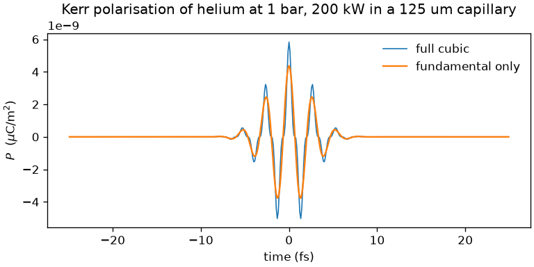
The two differ by the third harmonic, which is a quarter of the cubic’s amplitude for a monochromatic field and a tenth of its spectral power — the number the third-harmonic test asserts on both grids.
Labelled mixture responses#
A mixture binds each response to a stable component label. The electric field is
shared, while each plasma channel integrates its own exposure and neutral depletion.
Electron density and current use the sum of channel populations; ionisation loss
weights each newly ionised population by its own potential. Splitting a population
into identical labels therefore preserves the summed response to arithmetic error.
Kerr compilation forms sum(rho_s * gamma3_s) once per stage; a dispersive electronic
response keeps one channel per species instead, each with its own filters: the
polynomial sums them exactly, and the symmetric evaluator builds one filter from the
mixture’s Kerr diagonal at every stage
(mixtures and vectors). Raman amplitudes use
the responding species’ density, with the explicit total-density linewidth
approximation described in mixtures. A one-component material uses
exactly the arithmetic of a single-gas run.
Use responses_for(mixture, plasma=..., raman=..., thg=..., lambda0=...) when
constructing physics objects directly, or the per-label plasma, preionisation and
raman controls of prop_capillary, prop_waveguide and their Simulation
constructors. An explicitly selected unavailable response fails with the component’s
name; a zero-density component retains its label and contributes zero.
Vector molecular Raman is available on numpy_ref, numba_cpu and native (CPU, and the
CUDA and HIP builds) for the Cartesian field representations. The gas material
factories carry isotropic vibration and rank-two rotation; custom scalar models and
default silica require an explicit tensor declaration for vector use. See the
standalone Raman model and examples.