Absorbing boundaries#

Both axes of the grid are finite and periodic, because both are sampled for FFTs. Energy that reaches the edge of the frequency window or the edge of the time window therefore does not leave the simulation: it wraps around and aliases onto the rest of the field. Absorbing boundaries attenuate light near the edges to reduce these artefacts. Their finite strength and width must be checked for the actual calculation.

They matter whenever the physics genuinely reaches the edge of a window — soliton self-compression, modulation instability, a dispersive wave walking out of the time window at a hundred femtoseconds per metre. The rest of the time they should do nothing at all, and saying so is part of their job.

This page covers solprop.boundaries: why the absorber is a rate rather than a mask, how its spectral and temporal parts are applied, what it costs, and how to tell when it is too weak. It is for anyone whose pulse, or whose spectrum, reaches the edge of its window, and for anyone who wants to know what the collars do to a run that never gets there. The collars it works from are built by solprop.grid and described in grids and Fourier conventions; why the absorber is a rate, and where its temporal part is applied, are also recorded among the design decisions. Which runs carry an absorber, and how to change it, is near the end. Where solprop’s absorbing boundaries differ from Luna.jl’s, the differences are listed in Noteworthy differences from Luna.

Rates, not masks#

The simplest absorbing boundary multiplies the solution by a fixed collar profile W after every accepted step. The cumulative absorption is then Wⁿ, where n is however many steps the adaptive controller happened to take — a number derived from rtol. Two things follow, and both are wrong:

the answer depends on the tolerance. Tightening rtol does not approach a limit, it increases the absorption. Refining sixteen-fold erodes the spectral wings fifty-fold.
the taper is not a taper. At realistic step counts Wⁿ is a brick wall at the edge of the flat region, and that brick wall is the limit the scheme approaches. It erodes genuine spectral wings.

An absorbing boundary must instead be an absorption coefficient per unit propagation distance, so that traversing a distance L attenuates by a factor that depends only on L and not on how the solver chose to subdivide it. solprop converts each collar profile into one. The spectral collar becomes

\[ \alpha(\omega) = -\frac{2 \log W(\omega)}{\ell}, \]

the rate that reproduces one multiplication by the window over the reference length ℓ; the temporal collar becomes the bounded profile

\[ \alpha(t) = \frac{A\,(1 - W(t))}{\ell}, \qquad A = 12.6, \]

the complement of its window (solprop.boundaries.TEMPORAL_ALPHA_LENGTH). Why the two differ is below.

The factor of two, and where it goes#

α is a power absorption coefficient, as everywhere else in solprop: power falls as exp(−αz), the field as exp(−αz/2), and the linear operator carries −α/2 (the conventions §2). The factor of two in the spectral definition is exactly what makes

\[ \mathrm{e}^{-\alpha \ell / 2} = W, \]

so that propagating through one reference length ℓ applies the collar profile to the field precisely once. The reference length is ℓ = length / boundary_N by default: “apply the window boundary_N times over the whole propagation”, with boundary_N = 20. The strength of the absorber is then a physical distance rather than a step count.

Where each part goes is decided by what can be applied exactly:

part	mechanism	why
`α(ω)`	folded into the linear operator as `−α/2` before the cumulative operator is integrated	diagonal in ω, so the propagator applies it exactly over any sub-interval, at no cost
`α(t)`	the term `−α(t)E(t)/2` added inside every stage evaluation, masked to the active band	diagonal in t, so it cannot ride the propagator, and it belongs in the derivative so that the scheme integrates it at its own order
hard band limit	a 0/1 mask outside the active band	idempotent, and part of the definition of the band rather than an absorber

The hard limit sits outside the active mask ω_min/2 < ω < 1.1 ω_max, following the conventions §3. Putting it at the in-band mask instead would erase the collar the graded absorber acts on.

The two temporal schemes#

The temporal rate cannot be folded into the cumulative operator, and it cannot share the nonlinear polarisation’s transform either, because the UPPE prefactor is applied after that transform and the absorber is a rate on the field, not a polarisation. Two schemes represent it as a rate:

solprop.boundaries.nonlinear_absorber_term() — add −α(t)E(t)/2 inside every stage, with its own modal transform, masked to the active band. This is the default.
solprop.boundaries.apply_split_step() — multiply the modal time-domain field by exp(−α(t)h/2) once per accepted step, followed by the hard band limit, because the product in time spreads content into every bin (on a field grid, chiefly the DC). One batched transform pair per step; the factors telescope, so the total is a rate whatever the step layout. Selectable as absorber_scheme="split_step".

Why the term and not the factor. The split factor is exact for the absorber alone, but applying it once per step is a Lie splitting of a term that does not commute with the linear flow — and a Lie splitting is first order. Measured on an N = 3 soliton launched into its collar, at 100, 200 and 400 fixed steps against the same problem at 1600, with the bounded temporal profile solprop uses:

scheme	relative error	observed orders
`split_step`	1.7e-3 · 8.6e-4 · 4.3e-4	1.00 · 1.00
`nonlinear`	3.5e-9 · 2.2e-10 · 7.1e-12	4.02 · 4.95

So the split factor caps a fifth-order scheme at first order wherever the collar removes anything, and makes the absorbed energy a function of rtol — the very defect the rate form exists to avoid, one level up. The conclusion does not depend on the temporal profile. With the capped logarithm as the temporal rate (below) the same ladder reads 7.657e-4 · 3.845e-4 · 1.912e-4 (orders 0.99 · 1.01) against 2.939e-5 · 1.278e-6 · 1.789e-8 (4.52 · 6.16), and quadrupling the steps moves the energy the split factor removes by 6.5e-5 of itself and the in-stage term’s by 9.0e-10. The in-stage term’s errors are four orders smaller under the bounded profile because the term it integrates is not stiff there.

What the term costs. One extra modal transform per stage, and one thing that needs watching: it is conditionally stable. The collar’s largest rate becomes an eigenvalue of the linearised problem, so an explicit method needs h·α/2 inside its stability region — 3.3 for DOPRI5. solprop.boundaries.stable_step() returns the limit, and translation refuses a problem whose replayed schedule or step floor is already past it, with a TranslationError naming the limit, the step and the remedies, rather than letting it diverge. A replay cannot reject a step: one that diverges for another reason stops with a ConvergenceError at the first step whose error norm is not finite, naming the step and the position, rather than writing NaN planes.

from solprop.boundaries import absorber, stable_step

boundary = absorber(grid)                 # ell = length / 20 by default
stable_step(boundary.temporal_rate)       # the longest step that will not blow up

An adaptive run finds the limit for itself — the rate reaches its ceiling only at the very edge of the window, where the field is negligible — so it costs steps and not correctness, and with the bounded profile only on runs shorter than about 2 · boundary_N steps. With the capped logarithm as the temporal rate it would cost steps everywhere: a ceiling of 60/ℓ on the collar’s last samples reaches the error estimate long before the stability limit, and on a reduced four-mode resonant-dispersive-wave capillary case costs 40 % more steps than the split factor, where the bounded profile takes the split factor’s count, 456 against 459. The split factor’s unconditional stability is the one thing it is better at, and why it stays selectable.

The two agree to first order in the step and differ at second, by (αh/2)²/2 — which is what the tests assert, and what would be false if the factor of one half were dropped.

Geometry, and the collar that is not one#

The collar geometry comes from the grid: the spectral collar rises over [ω_min/2, ω_min] and falls over [ω_max, 1.1 ω_max]; the temporal collar is symmetric about zero, flat over the requested window or over all but 5 % of the realised window at each end if that is smaller, so each collar has a guaranteed minimum width of 5 % and can reach inside the requested window (grids).

That guarantee matters. A collar made only of the slack between the requested and the realised window — the flat region at ±trange/2 and the zeros at the ends of the axis — vanishes whenever the transform size makes the realised window equal to the requested one, the common case on a power-of-two grid: the temporal window is then identically one except for a single sample, and the grid has no temporal absorber at all. solprop.boundaries.absorber() refuses a collar whose edge spans fewer than four grid samples: below that the discrete profile steps rather than tapers, the rate jumps to its cap in one sample, and the boundary is the brick wall the rate form exists to avoid.

The spectral cap, α·ℓ ≤ 60, has two jobs. The collar reaches exactly zero at the band edge and −2 log 0 is an infinity, which would put a NaN into the operator; and in the interaction picture the right-hand side is back-propagated by exp(+αΔz/2), which must stay finite. At 60 the field is attenuated by exp(−30), about 10⁻¹³, over one reference length — far below anything a propagation can represent. The temporal profile needs no cap: it is bounded by construction at 12.6/ℓ, and every rate is still validated against the ceiling of 60.

Why the temporal rate is not the logarithm#

The obvious temporal rate is the same capped logarithm as the spectral one. That is the right rate for a window that rides the linear operator for free, and the wrong one for a term in every stage: the Planck window falls so steeply that −2 log W is above 12 over the outer 14 % of each edge, which carries 73 % of the edge’s integrated attenuation, and the cap of 60 that keeps −2 log 0 finite becomes the largest eigenvalue of the linearised problem — the stability limit of the in-stage term and, through the error estimate, its step count. Lowering the cap alone halves the attenuation, because so much of it sits under the cap.

The profile A(1 − W)/ℓ keeps the integral — A = 12.6 reproduces the capped logarithm’s 6.3 per collar width per reference length to a few per cent — with a largest rate a fifth of the logarithm’s, every derivative continuous, and the attenuation spread over the edge instead of piled at its end. Measured on the reduced resonant-dispersive-wave case above: 456 steps against 637, and the in-window field differs between the two profiles by 3e-3 in the fundamental and 2e-3 in the second mode, on a case that carries 6 % of its fundamental in the collar. A case that holds a twentieth of its input field in the collar — a reduced hydrogen-filled capillary supercontinuum case — changes in kind between the two profiles: when a run’s physics happens inside the absorber, the result depends on the absorber, and the time window has to be widened.

Walk-off#

An absorber doing its job is silent, so solprop.boundaries.warn_walkoff() says when it stops being strong enough. A packet whose group delay drifts by Δτ over the whole propagation crosses the temporal collar at Δτ/L seconds per metre, so it spends dt/(Δτ/L) metres at each sample and accumulates

\[ \frac{L}{\Delta\tau}\,\frac{1}{2}\int \alpha(t)\,\mathrm{d}t \]

nepers of field attenuation on the way through. Below log(10³) — the field down by a thousand, the power by sixty decibels — the packet reaches the edge of the window still alive, wraps around, and appears at the front of the time window as an alias.

The group-delay span is the caller’s, deliberately. A prediction from the group delay across the whole simulation band, which on a grid running to four microns is dominated by band edges carrying nothing but shot noise, fires on almost every run — and a warning that is usually wrong is one people learn to ignore. A caller who passes the span of the band it cares about does not have that problem.

import numpy as np
import matplotlib.pyplot as plt

from solprop.boundaries import absorber, split_step_factor
from solprop.grid import FieldGrid

grid = FieldGrid.from_limits(1.5, 800e-9, (90e-9, 4e-6), 400e-15)

fig, (ax_rate, ax_steps) = plt.subplots(1, 2, figsize=(9.5, 3.6))

# Only the trailing collar: it is 5 % of the window at each end, so the whole axis
# would show two vertical lines and nothing else.
twin = ax_rate.twinx()
ax_rate.plot(grid.t * 1e15, grid.t_window, color="0.5", lw=1.2)
ax_rate.set_ylabel("collar profile", color="0.5")
ax_rate.set_ylim(-0.02, 1.05)
for index, strength in enumerate((20, 60)):
    rate = absorber(grid, boundary_N=strength).temporal_rate
    twin.semilogy(
        grid.t * 1e15, rate, color=f"C{index}", label=f"boundary_N = {strength}"
    )
twin.set_ylabel("absorption rate (1/m)")
twin.set_ylim(1e-2, 1e4)
twin.legend(frameon=False, loc="upper left", fontsize="small")
ax_rate.set_xlabel("time (fs)")
ax_rate.set_xlim(178, 206)

# A point part way down the taper, where the collar profile is 0.9. As a rate the
# surviving field is exp(-alpha L / 2) whatever the step layout; as a per-step
# multiply it is 0.9^n, which is a different answer for every step count.
boundary = absorber(grid)
profile = 0.9
alpha = -2.0 * np.log(profile) / boundary.reference_length
distance = 0.3
counts = np.array([1, 2, 5, 10, 20, 50, 100, 200, 500, 1000])
as_a_rate = [
    float(np.prod(split_step_factor(np.array([alpha]), distance / n) ** n))
    for n in counts
]
ax_steps.loglog(counts, as_a_rate, "o-", label="as a rate")
ax_steps.loglog(counts, profile**counts, "s--", label="per-step multiply")
ax_steps.set_ylim(1e-20, 3.0)
ax_steps.set_xlabel("steps taken over 0.3 m")
ax_steps.set_ylabel("surviving field amplitude")
ax_steps.legend(frameon=False)

fig.tight_layout()

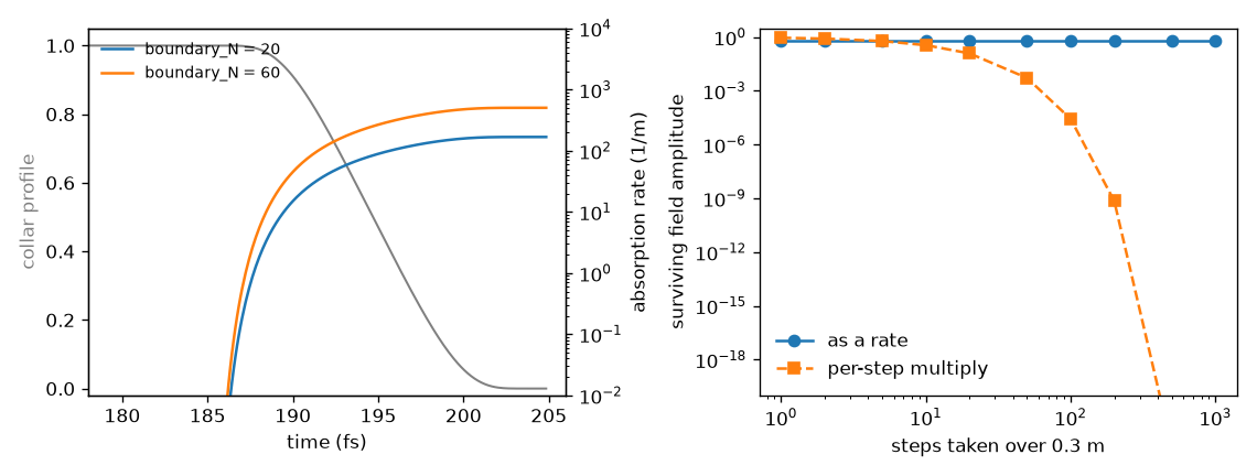
../../_images/boundaries-1.png — Left: the temporal collar of the RDW field grid and the absorption rate it becomes, for two absorber strengths. Right: the property the whole scheme exists for – the surviving field after 0.3 m is the same however that distance is subdivided, while a per-step multiply gives a different answer for every step count.#

Two lengths: the spectral rate and the in-stage collars#

A single length would set three things: the spectral collar’s strength, the ceiling 60/ℓ every rate is validated against, and the strength of the in-stage collars, the temporal 12.6 (1 − W(t))/ℓ and, on a spatial grid, the transverse 12.6 (1 − W(x, y))/ℓ (free-space propagation). The two kinds of rate are applied very differently. The spectral rate is diagonal in ω and rides the linear operator, where it is exact and free whatever its strength; the in-stage collars are explicit terms, and their largest rate bounds the step an explicit method can take (the stable step). A measurement that needs a strong spectral absorber should not pay for it in steps.

So Absorber carries two lengths (SEP 22 §4.6):

reference_length, ℓ, sets the spectral rate and its ceiling 60/ℓ;
collar_length, ℓ_c, sets the in-stage collars — the temporal one’s largest rate is 12.6/ℓ_c, and the spatial collar is 12.6 (1 − W)/ℓ_c — and their ceiling 60/ℓ_c. None, the default, means reference_length, and a value equal to the reference length is stored as None. in_stage_length returns the length in force.

Take a 1 mm sample whose measurement calls for a spectral power rate of 10⁷ m⁻¹. The default ℓ = 50 µm caps rates at 1.2 × 10⁶ m⁻¹, so a single length would have to fall to 6 µm; the spatial collar’s peak would rise from 2.5 × 10⁵ to 2.1 × 10⁶ m⁻¹ and its DOPRI5 stable step fall from 26 µm to 3.1 µm. With two lengths the spectral rate moves and the collars do not.

collar_length is whatever sets the temporal collar’s strength — boundary_N or boundary_length today. SEP 21, which owns the temporal collar, may parameterise that strength by a protected walk-off; the spatial collar follows the same length until its findings say otherwise.

A custom spectral absorber#

custom_absorber() adds a power rate of your own to a collar’s spectral rate:

from solprop.boundaries import absorber, custom_absorber

boundary = custom_absorber(grid, 1e7)                       # a scalar, 1/m
boundary = custom_absorber(grid, rates, collar=absorber(grid, boundary_N=60))
boundary = custom_absorber(grid, lambda omega: 1e6 * (omega > omega_cut))

The rate is a scalar, an array on the grid’s frequency axis or a callable of ω in rad/s; it must be finite and non-negative, and it is zeroed outside the collar’s band mask, where the operator is zero anyway. The collar is taken by value — None is absorber(grid), and any collar is accepted as it is, a spectral-only one included — and its temporal rates, band mask and in-stage strength are kept: the result’s collar_length is the collar’s own in_stage_length. Its reference_length stays the collar’s when the summed rate fits under the collar’s ceiling, and otherwise becomes 60 over the sum’s largest value, the longest length that admits it. The default collar already reaches its ceiling at the band edges, so any rate added there moves the reference length; the explicit collars never move. A zero rate returns the collar field for field, so its runs have the collar’s results and configuration hash.

The user’s rate is summed into the collar’s, so a diagnostic of the spectral collar’s absorbed energy reports the two together.

A spectral-only collar#

absorber(grid, temporal=False) builds a collar with the spectral rate and the band mask of a full collar and no temporal part: its temporal rates are zero arrays on both time axes and its record says temporal: False. Any collar whose temporal rates are all zero, however it was built, crosses the seam as no temporal absorber (temporal_rates()), so the kernels compile no temporal pass under either scheme: no in-stage term, no split pass and its transverse transform pair, and the first-same-as-last stage recycled. absorber_scheme is still recorded and applies to nothing, and its refusal of interpolated planes does not fire. The grid is unchanged. Measured on a Cartesian envelope grid of 192 × 192 × 300 with a spectral-only collar, the pass that compiling away removes cost 1.3–2.3 times a step on numba_cpu and 1.2–1.6 times on native CPU (SEP 22 §3; the phase-1 re-measurement is in its implementation record). Under the in-stage scheme the zero rate only added zeros, so a run is unchanged; under the split it differs by the transform pair’s rounding.

A spectral-only collar is passed as absorber=absorber(grid, temporal=False); a keyword that turns both soft collars off on the fibre entry points is SEP 21’s.

A transverse collar#

The collars above act on time, frequency and the transverse coordinates. A Cartesian run may also carry a ramp in the transverse wavenumber, SimulationSettings(transverse_absorber=TransverseCollar(strength)) (TransverseCollar, SEP 22): a power rate diagonal in \(k_\perp\), which rides the linear operator exactly, like the spectral rate, rather than the stages. It is a safety ramp at the grid’s largest wavenumbers, not anti-aliasing, and is independent of the Absorber and its lengths: grid sizing and the transverse safety ramp.

Which runs carry one, and how to change it#

entry point	absorber by default
`prop_capillary`, `prop_waveguide`, `Simulation.from_capillary`, `Simulation.from_waveguide`	the grid’s default collar, `absorber(grid)`: spectral and temporal, `boundary_N = 20`, applied in every stage
`prop_gnlse`, `Simulation.from_gnlse`	none
a `Simulation` built with its own `SimulationSettings`, and the free-space and planar entry points, which take one	none unless `SimulationSettings(absorber=...)` is given

The fibre entry points take absorber=: pass absorber(grid, boundary_N=60) for a stronger one, or absorber(grid, boundary_length=...) to fix the reference length ℓ directly. absorber=None there means “build the default”, not “no absorber”. To run without one, or with the split scheme, replace the simulation’s settings before its first translate() or run(); after it the translated problem is cached and an assignment that changes anything but the backend raises DriverError:

import dataclasses

simulation.settings = dataclasses.replace(simulation.settings, absorber=None)
# or: dataclasses.replace(simulation.settings, absorber_scheme="split_step")

On a spatial grid the same absorber also switches on the transverse collar (free-space propagation).

A worked example#

import numpy as np
from solprop.boundaries import absorber, apply_band_mask, apply_split_step, warn_walkoff
from solprop.grid import FieldGrid

grid = FieldGrid.from_limits(1.5, 800e-9, (90e-9, 4e-6), 400e-15)
boundary = absorber(grid, boundary_N=20)

# The spectral rate goes into the linear operator as -alpha/2. Here the temporal rate
# is applied to the time-domain field once per accepted step: the `split_step` scheme,
# which `absorber_scheme="split_step"` selects (the default applies it in every stage).
field = np.ones((1, 1, grid.n_t))
field = apply_split_step(field, boundary.temporal_rate, step=0.01)

# The hard band limit is a separate, idempotent multiply on the spectrum.
spectrum = apply_band_mask(np.ones((1, 1, grid.n_omega)), boundary.band_mask)

# And the run says so if the absorber is too weak for the walk-off it will produce.
warn_walkoff(grid, group_delay_span=1e-12)   # SolpropWarning: widen trange, or ...