Vector boundary response#

The electric field normal to a dielectric wall and the field tangential to it see different impedances. Retaining both gives separate TE and TM losses and can couple hybrid families. This chapter extends the mean-impedance coherent wall; the vector-wall worked example compares the two descriptions.

The vector boundary response#

The mean-impedance model uses one impedance-averaged condition: the wall is given a single \(k_{\rm eff}\), which is what a linearly polarised \(\mathrm{HE}_{1m}\) field sees on azimuthal average. The wall does not impose one condition. At grazing incidence it imposes two — the field tangential to the glass sees \(\partial_rE = ik_oE\) and the field normal to it sees \(\partial_rE = i(k_o/n_r^2)E\), with \(n_r\) the wall’s index relative to the core and \(k_o = k\sqrt{n_r^2-1}\) the transverse wavenumber in the glass — and those two differ by the whole index contrast. CoherentWall(impedance="te_tm") condenses both; the default impedance="mean" is the averaged block above. Use it for radially or azimuthally polarised light (\(\mathrm{TE}_{0m}\), \(\mathrm{TM}_{0m}\)) and whenever a hybrid mode’s partner family (\(\mathrm{EH}\) beside \(\mathrm{HE}\)) matters; the mode set it needs is set out under “Declaring one” below.

The name is the wall’s: "te_tm" gives the wall’s TE and TM fields their own impedances and adds no polarisation axis to the state, whose channels still carry one state component each, so a two-component state beside any wall is refused by name. The synthesis is a separate matter: a TE_0m, TM_0m or EH channel has both \(E_x\) and \(E_y\), and a supplied set given to prop_capillary resolves both, with or without a wall. The flow contracts the channel axis of the one-component state and never reads the synthesis, so every backend admits it beside two synthesised components. (Synthesising \(E_x\) alone would leave a TE_01 channel only 3/8 of its Kerr overlap.)

Near a Dirichlet wall the condensation is linear in the impedance \(1/k\), not in the admittance, so what enters is the matrix \(Z = \operatorname{diag}(1/k_{\rm TM},\,1/k_{\rm TE})\) in the \((\hat r,\hat\theta)\) components. Rotating it into a guide’s radial families is the whole of the vector boundary response. Because the wall is rotationally symmetric the total azimuthal order \(\nu\) is exactly conserved, and an order has at most two radial families: the transverse field of an order-\(\nu\) mode is a combination of the two circular components \(\hat e_\pm\), whose Cartesian angular harmonics are \(\nu\mp1\) and whose radial functions are therefore \(J_{\nu-1}\) and \(J_{\nu+1}\). Integrating \(Z\) over their angular patterns gives, for \(\nu \ge 1\),

\[Z = \bar z\,I + \delta\,\sigma_x,\qquad \bar z = \tfrac12\!\left(\frac1{k_{\rm TM}} + \frac1{k_{\rm TE}}\right),\qquad \delta = \tfrac12\!\left(\frac1{k_{\rm TM}} - \frac1{k_{\rm TE}}\right),\]

and for \(\nu = 0\) the same matrix diagonalised: \(\mathrm{TM}_{0m}\) is purely radial at the wall and sees \(1/k_{\rm TM}\), \(\mathrm{TE}_{0m}\) is purely tangential and sees \(1/k_{\rm TE}\), and the two do not couple at all.

Three things follow, and they are what a vector wall is for.

The average is recovered, not assumed. \(\bar z\) is exactly the scalar block’s \(1/k_{\rm eff}\), because \(v_{\rm HE}\) is the arithmetic mean of \(v_{\rm TE}\) and \(v_{\rm TM}\) — the two impedances this block carries are this package’s own Marcatili cladding terms for a \(\mathrm{TM}_{0m}\) and a \(\mathrm{TE}_{0m}\) channel. The impedance average is the right one. Averaging the admittances instead gives a hybrid loss too low by \(4n_r^2/(1+n_r^2)^2\), which is 0.872 for a silica wall. In the continuum limit, Andreasen and Kolesik’s field average, their Eq. (15) (Phys. Rev. E 87, 053303 (2013)), amounts to that admittance average; this is solprop’s reading of their equation, not a statement of the paper, whose own test on a finite grid agrees well with a resolved cladding.
\(\mathrm{TE}_{0m}\) and \(\mathrm{TM}_{0m}\) keep their own losses, a factor \(\varepsilon\) apart. No impedance-averaged block, and no two copies of one, can produce that.
The anisotropy \(\delta\) couples the two hybrid families of every order \(\nu\ge1\) — \(\mathrm{HE}_{1m}\) to \(\mathrm{EH}_{1m}\), \(\mathrm{HE}_{2m}\) to \(\mathrm{EH}_{2m}\) — and it is not a perturbation: \(\delta/\bar z = (n_r^2-1)/(n_r^2+1)\), which is 0.357 for silica against helium at 800 nm.

The condensation itself is then the scalar one made rank two. Truncating the Mittag-Leffler expansion of the exact recurrence \(qJ_{p+1}(q) = (p - i\eta)J_p(q)\) family by family and eliminating the boundary coordinate gives

\[L_N = -\operatorname{diag}(u_m^2) + VSV^{T},\qquad S = \left(C - i\,aZ^{-1}\right)^{-1},\qquad C = \operatorname{diag}(2N_f + p_f),\]

with one boundary-trace column of \(V\) per family and \(G = iL_N/(2ka^2)\) as before. The truncation constant carries the family’s Bessel order \(p_f\) beside the \(2N_f\) of the scalar block; without it the condensed eigenvalues stop converging to the exact roots, and it is invisible in the scalar case only because the \(\mathrm{HE}_{1m}\) family’s order is zero. That is also why a vector block of the \(\mathrm{HE}_{1m}\) family alone is the scalar block to the last bit rather than a second model of the same thing.

Declaring one#

A vector wall is declared by wall=CoherentWall(impedance="te_tm") beside a supplied mode set that is one azimuthal order, family by family: the hybrids of azimuthal index \(n = +\nu\) followed by those of \(n = -\nu\), each contiguous from \(m = 1\), or for \(\nu = 0\) the \(\mathrm{TE}_{0m}\) and \(\mathrm{TM}_{0m}\) families. A negative azimuthal index is this package’s spelling of the \(\mathrm{EH}\) family, and its channels label themselves that way. The figure below builds the \(\nu = 1\) set \(\mathrm{HE}_{11}, \mathrm{HE}_{12}, \mathrm{EH}_{11}, \mathrm{EH}_{12}\).

import warnings

import matplotlib.pyplot as plt
import numpy as np

from solprop.boundaries import absorber
from solprop.driver import prop_capillary
from solprop.grid import FieldGrid
from solprop.modes import CoherentWall, MarcatiliMode

length, steps = 2e-4, 10
grid = FieldGrid.from_limits(length, 800e-9, (400e-9, 1.6e-6), 300e-15)
# The order nu = 1: the J_0 family and the J_2 family, contiguous from m = 1.
modes = [
    MarcatiliMode(50e-6, n=order, m=radial + 1)
    for order in (1, -1)
    for radial in range(2)
]                                  # HE_11, HE_12, EH_11, EH_12

def run(wall):
    # A marginal geometry on purpose, and a band past the fitted ranges: both say so.
    with warnings.catch_warnings():
        warnings.simplefilter("ignore")
        return prop_capillary(
            50e-6, length, "He", 1.0, lambda0=800e-9, grid=grid,
            # A collar weak enough that twenty-micrometre steps are stable.
            absorber=absorber(grid, boundary_length=1e3),
            fwhm=30e-15, energy=1e-9, modes=modes, n_save=6,
            backend="numpy_ref", wall=wall, plasma=False, raman=False,
            dz_max=length / steps, dz_init=length / steps,
        )

walled, plain = run(CoherentWall(impedance="te_tm")), run(None)
print(walled.metadata.modal["flow"]["model"], walled.metadata.modal["basis"])

fig, ax = plt.subplots(figsize=(6.4, 3.8))
labels = ["HE_11", "HE_12", "EH_11", "EH_12"]
for handler, style, name in ((plain, ":", "wall=None"), (walled, "-", "te_tm")):
    planes = handler.planes()
    z = np.array([plane.z for plane in planes]) * 1e6
    energy = np.array(
        [np.asarray(plane.stats["energy"]).reshape(4, -1)[:, 0] for plane in planes]
    )
    for channel in range(4):
        ax.semilogy(
            z, np.maximum(energy[:, channel] / energy[0, 0], 1e-60), style,
            color=f"C{channel}", label=f"{labels[channel]}, {name}",
        )
ax.set_xlabel("z (um)")
ax.set_ylabel("fraction of the launched energy")
ax.set_ylim(1e-55, 3.0)
ax.legend(frameon=False, fontsize="small", ncol=2)
fig.tight_layout()

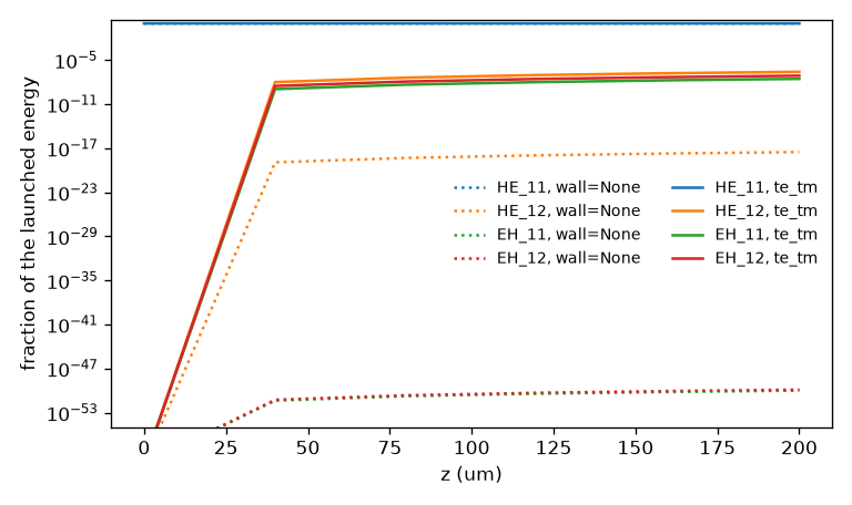
../../_images/modes-vector-wall.png — The wall’s anisotropy converts between the two radial families of one azimuthal order. Ten fixed steps of 20 micrometres of a 50 micrometre helium-filled bore, launched into HE_11 alone, with the fraction of the arriving energy in each channel. The vector block leaves 2.8e-8 in EH_11; the uncoupled route leaves 1e-50 there, and the scalar block cannot carry the set at all.#

A supplied mode set is the run’s geometry: its modes keep their own radius, model, loss and cladding. prop_capillary’s positional radius must therefore agree with every mode’s core radius along the run – a different bore, or a taper beside a constant-bore set, is refused by name – and a model, loss or cladding declared away from its default must be the modes’ own, or it is refused rather than ignored. The vector wall: two impedances, two families, one conversion sets out each family’s own loss, the \(\mathrm{HE}_{11}\to\mathrm{EH}_{11}\) conversion and its \(\delta^2\) scaling.

Either family may be retained alone — that is how the single-family loss limits are taken, and how a \(\mathrm{TE}_{0m}\)-only run is written — in which case the block carries no conversion and says so in its record, whose model reads "te_tm impedance coherent wall" and whose gauge_id names the order.

Every refusal of the scalar block is a refusal of this one, at the same doors. Two sets are refused for the physics rather than for the scope: a set spanning two azimuthal orders, which is two blocks and not one, and a set whose families disagree about the polarisation angle \(\phi\), which does not close — the boundary form between two families at angles \(\phi_A\) and \(\phi_B\) carries \(\cos\nu(\phi_A-\phi_B)\), so a relative angle couples each family to both partners of the other.

What it is checked against#

The single-family limits are checked against the exact vector boundary roots — the full Maxwell match of \(E\) and \(H\) to outgoing Hankel functions in the cladding, with the hybrid cross term, solved by an independent reference code that knows nothing about any condensation. For a 150 µm bore the block reproduces those roots to between 5e-6 and 5e-5 at 800 nm and between 3e-4 and 3e-3 at 6 µm, for \(\mathrm{TE}_{0m}\), \(\mathrm{TM}_{0m}\), \(\mathrm{HE}_{1m}\) and \(\mathrm{EH}_{1m}\) alike, which is the same size as this package’s own Marcatili formula’s departure from the same roots. The coupled eigenvalues are checked against the exact two-family root equation \(\det[\operatorname{diag}(T_{p_A},T_{p_B}) - iaZ^{-1}] = 0\), which they approach as \(1/N\). The coupling is checked against something that does not contain it: the exact \(\nu = 1\) Maxwell roots resolve the hybrid cross term, and the coupled block’s eigenvalue nearest \(\mathrm{EH}_{11}\) departs from them 3.2 to 6.3 times less than the same block’s with the impedance averaged (\(\delta = 0\)), at 800 nm and 6 µm. The mixed-family coupling has not been compared with a resolved-cladding Maxwell solve excited in a mixed-family state, which would be the stronger check. And the boundary form itself is checked by integrating \(\int_0^{2\pi}[Z_{rr}P_fP_g + Z_{\theta\theta}Q_fQ_g]\,\mathrm{d}\theta\) over the fields field() implements, which fixes every sign in the block — including the \(J_{-p} = (-1)^pJ_p\) of a family built from jv(n-1, ·), which flips the coupling of every even order.

The conversion is small on a straight bore and it is real. Ten steps of 20 µm of a 50 µm helium-filled bore, launched into \(\mathrm{HE}_{11}\), leave 2.8e-8 of the arriving energy in \(\mathrm{EH}_{11}\) where the uncoupled route leaves 1e-50, and the transfer scales as \(\delta^2\): moving the cladding index from 1.45 to 1.21 reduces \(\delta\) by 1.542 and the conversion by 2.378, against the predicted 2.377.

On a guide that varies along z#

A taper or a pressure gradient beside impedance="te_tm" takes the route of A guide that varies along z unchanged but for two things: the frozen block is this one, and so is the connection. A taper moves the radius and nothing else, and every channel’s field is a radial function of \(r/a\) times an angular pattern that does not depend on \(a\). So:

within a family the connection is the \(\mathrm{HE}_{1m}\) formula with that family’s own Bessel order \(p\) — its zeros \(u_m\) of \(J_p\) and its slope signs \(s_m = \operatorname{sgn}J_{p+1}(u_m)\), since \(-J_p'(u_m) = J_{p+1}(u_m)\) —

\[C_{mn} = \frac{a'}{a}\,\frac{2s_ms_nu_mu_n}{u_m^2-u_n^2}\quad(m\ne n);\]

the implemented sign of a family built from jv(n-1, ·) enters as \(s_ms_n\) and cancels;
between the families it is exactly zero: \(\langle\psi^A_m|\partial_z\psi^B_n\rangle\) is a radial integral times the two angular patterns’ overlap, which is \(\int\cos 2\nu\theta\,\mathrm{d}\theta = 0\) for the two hybrid families of an order and a pointwise zero for \(\mathrm{TM}_{0m}\) against \(\mathrm{TE}_{0m}\).

Both are measured, not assumed: the \(z\) derivative of the fields field() implements, paired over the cross-section by quadrature, reproduces each family’s matrix to \(1.7\times10^{-11}\) of its size (the difference step’s rounding) and leaves the cross-family entries at \(8\times10^{-14}\), for \(\nu = 0, 1, 2\) and a rotated \(\nu = 3\) pair. The connection is stored in the true-power amplitude like the scalar one, \(\sqrt{w_n/w_m}\,C_{mn}\) with each channel’s own weight, and each channel keeps its own normalisation on the diagonal. So on a taper, as on a straight bore, only the wall’s anisotropy moves power between the families: halving \(\delta\) quarters the \(\mathrm{EH}_{1m}\) share to 0.15 %, and a \(\mathrm{TM}_{01}\) launch leaves the \(\mathrm{TE}\) family at \(10^{-52}\) while the connection moves 11 % of it into \(\mathrm{TM}_{02}\). Against an independent solve in the true-power amplitude whose connection is the measured matrix rather than the formula, ten steps of the 50 to 40 µm taper agree to \(1.2\times10^{-8}\) on every channel ratio and converge at fifth order. A single \(\mathrm{HE}_{1m}\) family under the TE/TM wall is the scalar taper to rounding, and method="cf4" is admitted here too. numba_cpu and the native CPU backend run the vector wall on a taper as well, within 1e-11 of the reference’s final plane after ten steps (the frozen-residual method; CF4 stays numpy_ref’s).