Choosing a stepper#
solprop has three integrators, chosen with integrator=; this page is their overview.
Multistep(), the default, is an exponential Adams method: one source evaluation per
accepted step, a history of the last few, and an order it chooses between one and five
(the Adams integrator). RungeKutta() is the interaction-picture
Dormand–Prince 5(4) pair: six evaluations with FSAL reuse, seven otherwise,
and no multistep history
(the Runge–Kutta integrator). Both integrate the
represented diagonal linear flow exponentially and share the error norm and
controller. Coupled flows have additional restrictions and residual errors;
check the limitations for the chosen formulation.
LowStorageRungeKutta() is a third, for fixed-step runs whose state is too large for
either: classical RK4 in the interaction picture, replaying a prescribed schedule in
three copies of the state, with no error estimate (below).
This page sets out what decides between them, what was measured, and how to recognise
a problem that wants another one.
The short answer#
Keep the default for almost everything, and in particular wherever a source evaluation is the expensive part of a step: several modes, ionisation and plasma, Raman, a spatial state (radial, Cartesian, line or planar), a gas gradient or a taper, a time-dependent Schrödinger equation. There it takes two to fourteen times fewer calls than the Runge–Kutta march and, measured, up to six times less time.
Choose integrator=RungeKutta() when
the source is cheap and the state small — a single-mode envelope (GNLSE) supercontinuum: the Adams method still takes three to four times fewer calls, but a call costs less than a Runge–Kutta step’s own linear work, and the Runge–Kutta march is 1.2 to 1.4 times faster on
numba_cpu(level on native CPU);the state is too large for the Adams history (large problems);
an explicitly integrated damping term binds the step: a strong in-stage collar the field reaches, or a replayed schedule whose steps are long against it — the Adams method’s negative-real stability interval is 0.09 to 1 by order, DOPRI5’s 3.3 (stability);
a handful of fixed steps is all a run takes: the Adams history starts at order one at the start of a schedule (a resume continues it on the CPU backends, from the snapshot the output keeps);
the backend is not
numpy_ref,numba_cpuornative.
Choose integrator=LowStorageRungeKutta() with a schedule= when the state is too
large for RungeKutta()’s stage rows and the run is a fixed-step one whose accuracy you
calibrate on the observable that matters (the low-storage march).
Within Multistep(), the interaction formulation (formulation="interaction") is the
alternative where the source is linear in each weak bin’s own field, as beside the
modified noise (which formulation suits which source).
What decides#
What a call costs against what a step costs. Every step of either integrator also pays fixed work that does not depend on the source: propagating the state, forming the error norm, the controller, landing. The Runge–Kutta march spreads that over six calls; the Adams method pays it for each call, and adds its history’s arithmetic. When a call dominates — a multimode transform pair, an ionisation rate, a Raman convolution, a transverse transform — fewer calls is less time, nearly in proportion. When a call is a few fast Fourier transforms of a single mode, the step’s own work weighs as much, and three times fewer calls can be slower. The compiled backends make calls cheap, which is why the ranking is measured per backend rather than read off the call count.
How complicated the nonlinearity is. A richer response costs more per call, which favours the Adams method, and its dynamics decide how far each step can go. The exponential formulation integrates a driven source — the four-wave mixing, Raman and plasma terms that build a dispersive wave or a continuum — at any linear phase per step, where the interaction picture’s history limits a step to a linear phase of about one in the populated bins. That is why it leads most on the gas-filled capillaries with ionisation (5.5 to 5.8 times faster than the Runge–Kutta march on the full RDW case, with twelve to fourteen times fewer calls) and on the Raman-active multimode launch. A source linear in a weak bin’s own field rotates with that bin’s free phase and favours the interaction picture; on real problems it lives in the dark wings (weak wings).
How smooth the dynamics are, and how tight the tolerance. The Adams method takes
more, shorter steps than the Runge–Kutta march at the same tolerance, each one call.
Smooth propagation at tight tolerance raises its order and lengthens its steps; abrupt
events — a fission, a kink in a profile — lower the order for a while. rtol means
something different to each integrator, so compare their errors, not their
tolerances. At rtol of 5e-2 or more the Adams method is unreliable and warned on.
How long the run is, and how many. A run’s first few steps rebuild the history from
order one, a fixed cost that a short run feels most. A single short run hardly matters;
in a scan of thousands, measure one point with each integrator before choosing, and
spread the points over a Pool of one-thread workers, which scales with the cores:
batching in lockstep buys nothing on the CPU and about 1.1 times on a GPU
(scans).
Planes. Both integrators interpolate save planes inside their steps
(interpolate_planes=True) at the step’s own order and no call; landing on them stays
the default, and with many planes the Adams method’s saving grows, since landing caps
its steps.
Measured#
Indicative ratios at matched error against a converged reference, one thread on a shared Darwin/arm64 workstation (the gallery below has every point, and the devices; the benchmark notes say how to read such ratios). Ratios are the Runge–Kutta march’s time over the default’s: above one, the default is faster.
case |
the source |
calls, |
time ratio, |
time ratio, native CPU |
|---|---|---|---|---|
full RDW capillary (four modes, ionisation, gas gradient) |
expensive, varying |
12 to 14 : 1 |
5.5–5.8 |
6.1–6.3 |
CtC launch (six modes, Raman) |
expensive |
2.3 to 3.7 : 1 |
2.0–3.2 |
2.0–3.3 |
radial focusing beam, filament with ionisation |
spatial |
2.5 to 6 : 1 |
1.2–2.4 |
1.3–2.2 |
Cartesian focusing beam (48 × 48) |
spatial |
3 to 6 : 1 |
0.9–2.0 |
1.2–2.4 |
full canonical capillary (one mode, ionisation, gas gradient) |
moderate, varying |
1.8 to 2.4 : 1 |
1.0–1.3 |
1.1–1.45 |
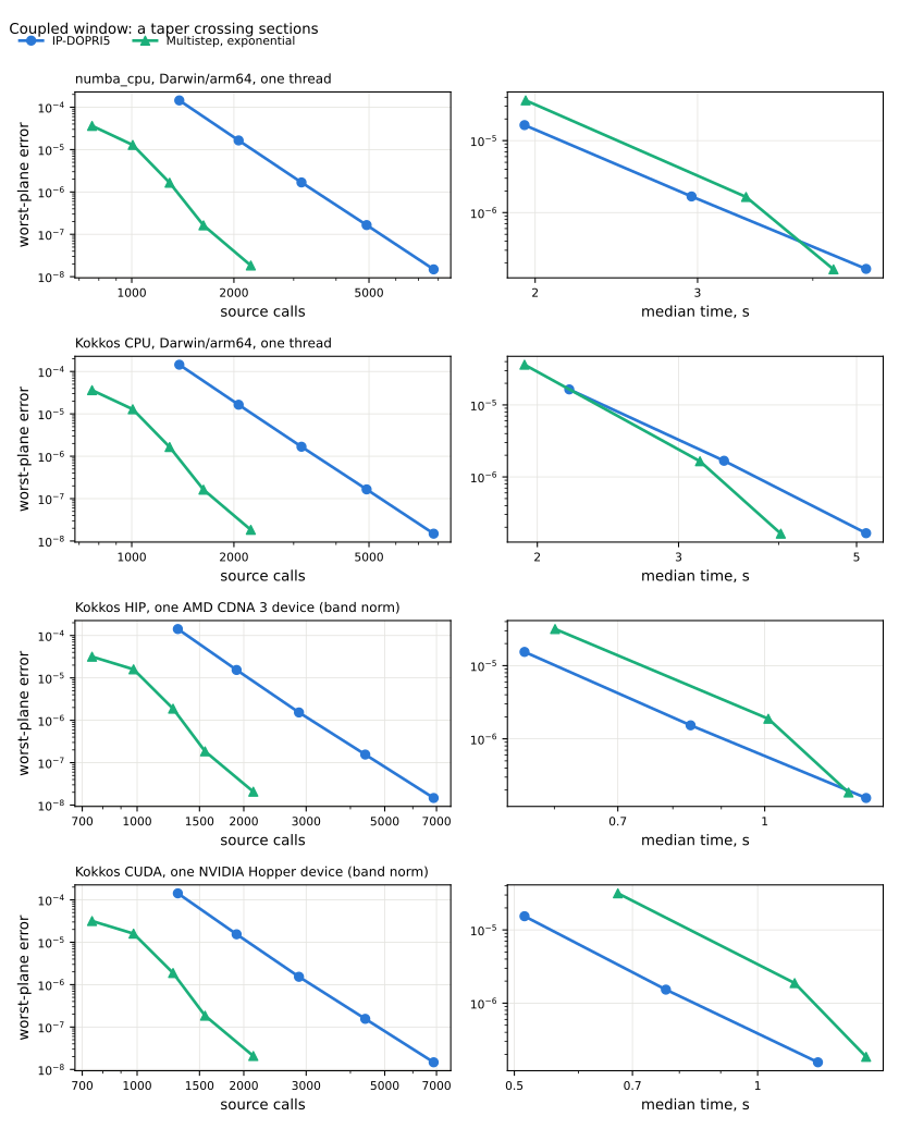
coupled flows: a coherent wall, a taper |
cheap, coupled |
1.8 to 4 : 1 |
0.6–1.4 |
0.7–1.7 |
line and planar self-focusing |
cheap, spatial |
2.4 to 6 : 1 |
0.8–1.8 |
0.9–2.3 |
GNLSE supercontinuum window |
cheap, one mode |
3.6 to 4 : 1 |
0.7–0.8 |
1.05–1.1 |
Below one, the Runge–Kutta march was faster: on the GNLSE window on numba_cpu, at
the tightest targets on the line, planar and radial-aperture cases, and at one or two
targets of the coupled taper and the Cartesian focus.
On data-centre AMD and NVIDIA GPUs the ranking is broadly the same: the exponential formulation was 4.4 to 4.8 times faster on the RDW capillary, 1.5 to 2.5 times on the CtC launch and the Cartesian focus and 1.1 to 1.3 times on the 512-node filament, while the Runge–Kutta march led on the canonical capillary and the coupled wall, by 1.25 to 1.9 times, because a device’s fixed cost per step is larger. These device ratios were measured with the error norm over the requested band rather than the whole active band, under which the Runge–Kutta march pays up to a fifth more calls on the capillaries.
Large problems: memory#
Most problems fit many times over, and memory need not enter the choice. It does when the state is large: a fine Cartesian grid, many modes over a wide window, a large batch on a device. The Adams history keeps further copies of the state beside what the march already holds — its source samples and, with a varying operator, the states and rates of its compensation:
backend |
history, copies of the state |
|---|---|
|
7; 21 with a varying operator |
|
7 in the interaction picture; 16, or 30 with a varying operator, in the exponential one |
|
29; about 60 with a varying operator |
What that adds depends on the rest. On a capillary the operator tables dominate, a
hundred to several hundred copies of the state, and the history adds 8 to 55 %. On a
Cartesian free-space grid the Runge–Kutta march holds 15 (native) or 16 (numba_cpu)
copies, by the backends’ ledgers, and the default 32 (numba_cpu) to 44 (native): two
to three times the memory. The low-storage march holds four or five:
integrator, on a Cartesian free-space grid |
copies of the state |
|---|---|
|
20 ( |
|
13 ( |
|
5 with the half-step flow tabulated, 4 recomputed; one more with the |
At 768 × 768 columns and 600 bins one copy is 5.3 GiB: 26 GiB under the low-storage
march, against 79 or 84 GiB for the Runge–Kutta march and 232 GiB for Adams on the native backend. The estimate is made
before anything is allocated (solprop.backends.memory.estimate_memory(),
group adams_history). A run that would fit with RungeKutta() but not with its
history is refused before it starts, naming RungeKutta(): against the machine’s
memory less a fifth when no budget is declared, and on a device against four fifths of
its free memory. A declared memory_budget or SOLPROP_MEMORY_BUDGET is admitted as
declared (execution resources).
The low-storage march#
LowStorageRungeKutta() is the classical fourth-order Runge–Kutta method in the
interaction picture anchored at each step’s midpoint, Hult’s RK4IP
(SEP 24). Only
forward half-step flows are applied, and on a constant operator one factor
\(e^{hD/2}\) serves every one of them. Each slope is folded into a running sum as soon as
it is produced, so beside the source pipeline’s scratch a step needs three copies of
the state: the state itself, overwritten in place, an accumulator and the next stage’s
input. Each step makes four source evaluations.
What it costs and what it gives up. It replays a prescribed schedule and nothing
else, so it needs schedule= (FixedSchedule.uniform(...) for plain fixed steps). It
has no embedded error estimate: every step’s recorded norm is 0.0, meaning “not
estimated”, and the run’s closing line says so. Its accuracy is the schedule’s,
measured on the observable with three-level Richardson calibration
(fixed schedules), which is also what makes
it the right tool for a weak band under a strong pump: the whole-field norm an adaptive
march controls is blind to a band holding a small fraction of the energy. Fourth order
needs more steps than fifth asymptotically; on stiff problems DOPRI5 measures about
fourth order at fixed step too, so compare the two at equal error, not at equal step.
What it refuses, by name and before anything is allocated: no schedule,
interpolate_planes, a coupled linear flow, the TDSE response, and a step past RK4’s
negative-real stability interval beside an in-stage collar, \(h\alpha_\max/2 \le 2.785\)
against DOPRI5’s 3.3 (about 45 steps over a run with the default temporal collar). A
Every backend runs it, on every route it admits it on, and backend="auto" resolves
as for any integrator: the native backend when it is installed, otherwise numba_cpu. On
numba_cpu the four passes are compiled register kernels with none of the Runge–Kutta
march’s buffers; on the native backend a step is one native call making the same four passes in
the backend’s own memory, and a plane that keeps no field holds its state there too.
Without an in-stage collar each pass writes the next one’s input straight into the
transverse scratch, so the stage register is not held either. On a Cartesian Kerr beam
the march
took 1.7 to 1.8 times less time per step
than the IP-DOPRI5 replay on numba_cpu, and
1.8 to 2.0 times less
on native CPU, in a quarter of the memory; what both marches spend is mostly the
source evaluation itself. The compiled backends do not form the stiffness indicator
below, so the warning is numpy_ref’s alone.
What a failure costs. Because each step is accepted in place, an exception or a
signal between a step’s first source evaluation and its commit leaves a state that is
neither end of the step. The backend then refuses to be observed or stepped until a
state is loaded again, and the run writes no terminal checkpoint, saying why: the file
ends at its last saved plane, from which resume=True continues, and step_planes=k
bounds the loss to k steps. A last plane that kept no field is held by the backend,
one more copy of the state, and checkpointed instead
(field retention). A field that diverges is caught on the accepted state, in
flight, with the same consequence. The march also watches its own stiffness: when the
indicator \(h\rho\) of SEP 24 §6.3 passes 2.785 on a step – strong plasma loss near
the stability limit – it logs a warning.
The flow. propagator_mode="tabulate", the default ("auto") for a constant
operator, holds one copy of \(e^{hD/2}\), reused while the step stays within eight ulps of
the step that built it; "recompute" forms it in each pass instead, the default for a
varying operator. The two agree to rounding. The free-space and planar kinds admit the
table under this march only.
Recognising the regime#
Stability-limited history. Many rejected trials, or the order falling to one or two while the error estimate stays small: a stiff term the explicit history integrates (an in-stage absorber, a strong plasma term) limits the step, not accuracy. Use the split-step collar where the pulse never reaches the collar (stability), or
RungeKutta().Reference-limited error. Errors that stop falling as
rtoltightens: below the reference’s own refinement (the dotted floor in each figure), nothing is resolved.Source-limited accuracy. The error is set by the response model’s own discretisation (a transverse quadrature, a TDSE grid); a tighter
rtolbuys calls, not accuracy.Dark wings. A total-field error that stays well above
rtolat tight tolerances while the populated bins follow it: free radiation far below the peak, which the exponential formulation integrates loosely (weak wings). Score the populated band, or take the interaction formulation if those bins matter.
The gallery#
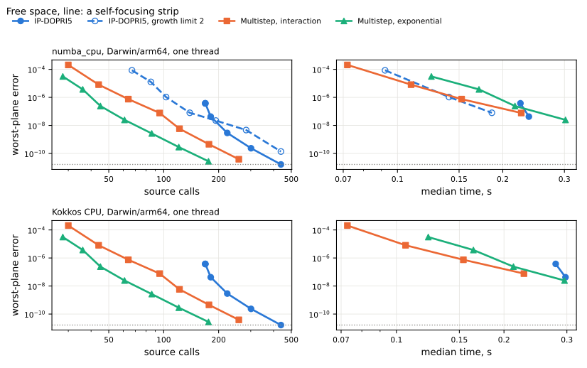
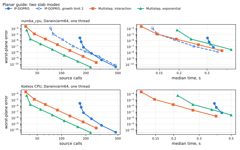
Each figure pairs, per backend, the case’s worst-plane error against (left) source
calls and (right) the median of interleaved timed rounds; every ladder point is drawn
against calls and only the timed points against time. The dotted line is the
reference’s refinement. Errors are scored per case: the
complex field and the weak band for the fibres and capillaries, the field in the scored
band for free space. IP-DOPRI5 is RungeKutta(); “Multistep, exponential” is the
default and “Multistep, interaction” its other formulation. “IP-DOPRI5, growth limit 2”
is IP-DOPRI5 allowed to grow a step by up to twice the last, as the Adams march is,
beside the default controller’s 1.1.
CPU timings are one thread on a shared Darwin/arm64 workstation, compared within one process; the device timings are the native HIP build on one data-centre AMD GPU and, for six cases, the native CUDA build on one data-centre NVIDIA GPU, with the error norm over the requested band; the CPU points use the default norm over the whole active band. Each figure’s points are in the CSV beside it.
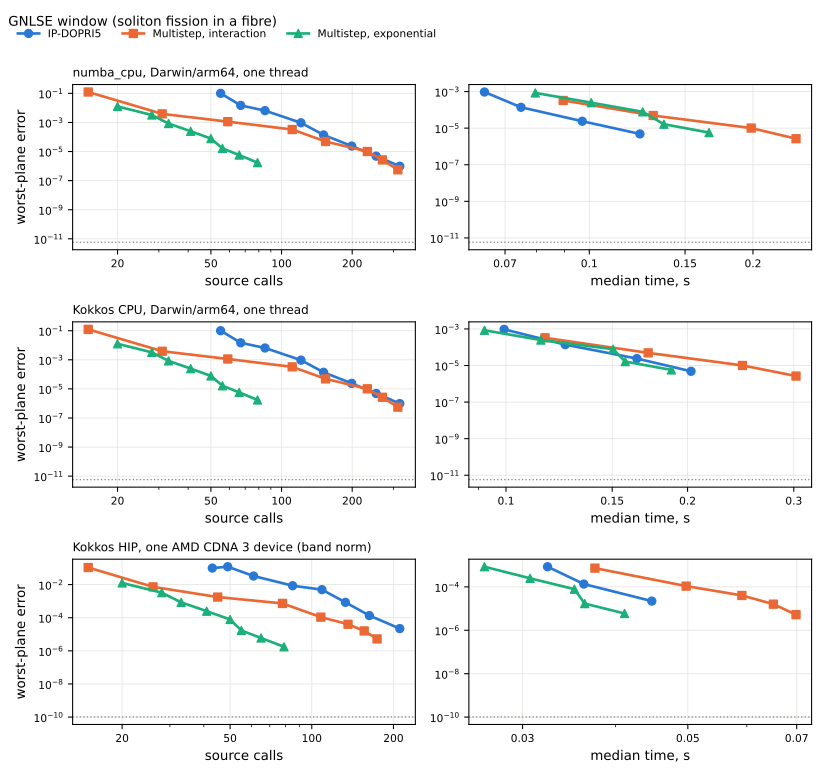
The GNLSE window: soliton fission in a fibre (envelope, one mode).
CSV#
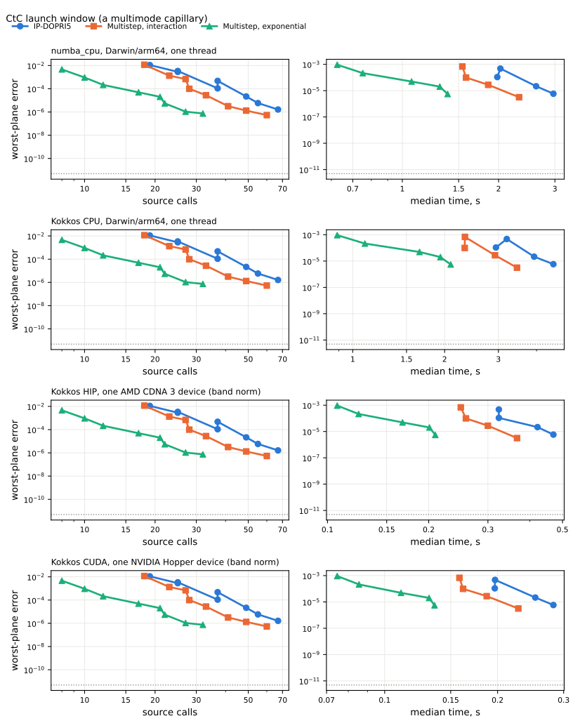
The CtC launch window: a multimode capillary, the expensive-source regime.
CSV#
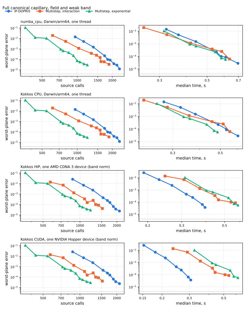
The full canonical helium capillary (4.2 m, steady fill), scored on the field and the
weak band. CSV#
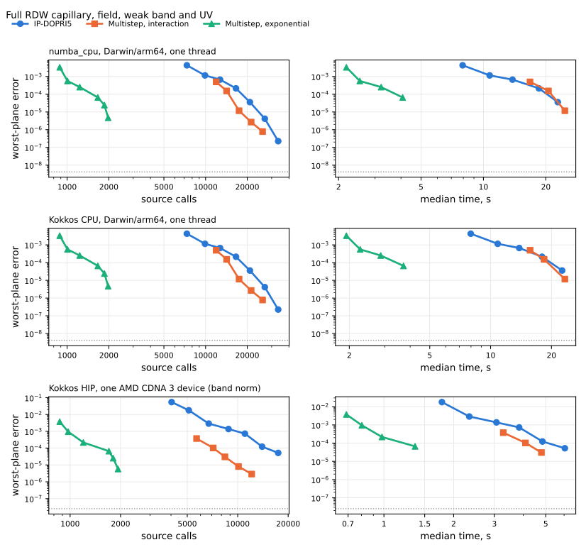
The full RDW capillary, scored on the field, the weak band and the UV.
CSV#
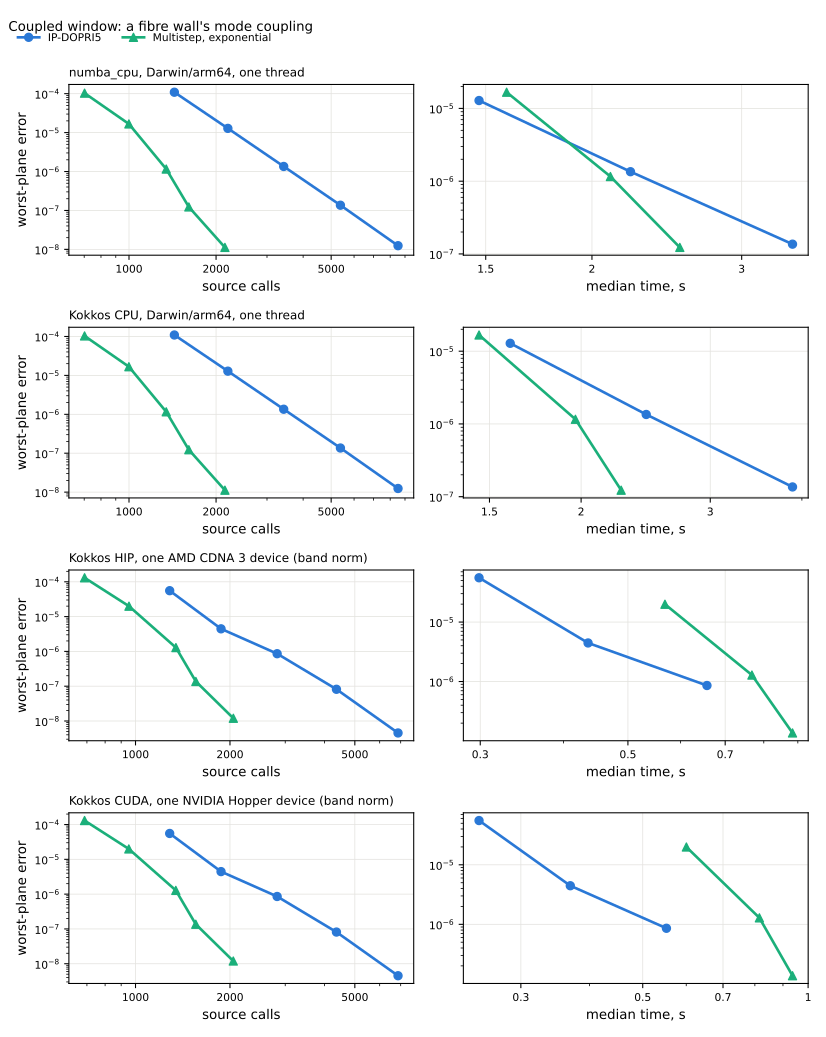
A coupled flow: a coherent capillary wall’s mode coupling.
CSV#
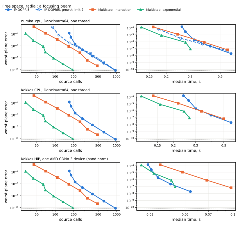
Free space, radial: a beam self-focusing at 0.9 of the critical power over 8 cm.
CSV#
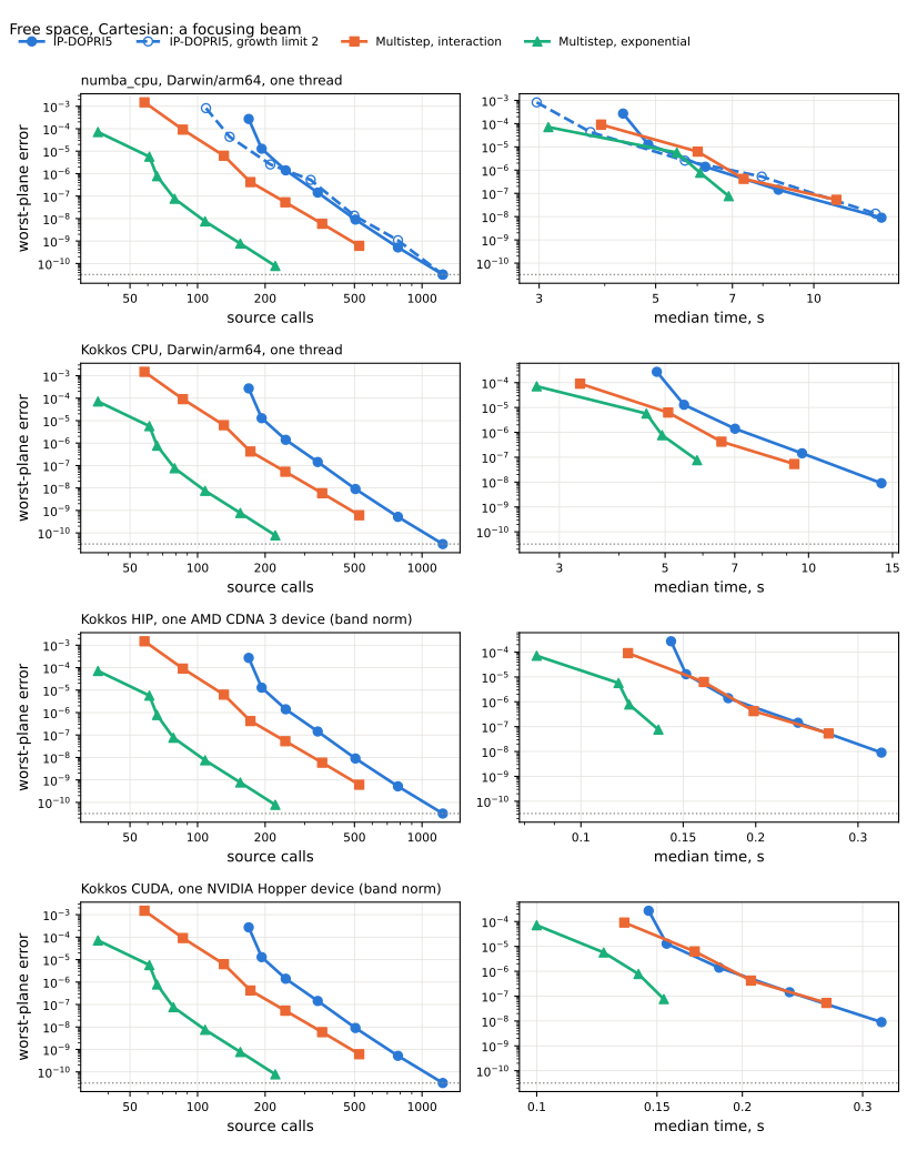
Free space, Cartesian (48 × 48): the same focusing beam.
CSV#
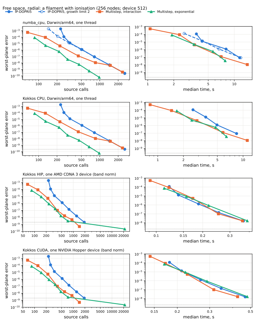
Free space, radial: a filament at three times the critical power with ionisation (256
nodes on the CPU; 512 on the device). CSV#
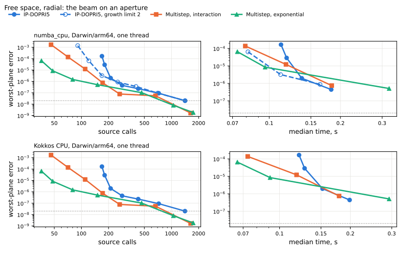
Free space, radial: the focusing beam on a 0.3 mm aperture.
CSV#
The qualification on this page was proposed and carried out by SEP 16.