Materials: gases, metals and glasses

Material data determine the refractive index, nonlinear response and losses of a calculation. Check the wavelength range, pressure, temperature and physical model against the observables you want to predict. A spectrum can extend into a region where the propagation is numerically resolved but the material data are uncertain.

Start with the catalogue below, then use material selection to inspect or change a model. The material-choices tutorial shows how to compare choices and read their records. Gas mixtures combines populations; solid guides use bulk glass data together with a mode model. General second-order (\(\chi^{(2)}\)) propagation and a general anisotropic crystal response are not modelled.

solprop keeps no material database of its own. Every built-in gas, solid and response comes from the curated package optmat (SEP 3): an omitted selection means MaterialSelection(), optmat’s recommended model of every family, and materials from optmat says what that resolves to. What solprop keeps is the propagation physics (linear density scaling, the mixture rule, the flow problem, the mode equations) and the types a caller’s own data take.

The built-in gases are thirteen: the noble gases He, Ne, Ar, Kr and Xe; the molecules N₂, H₂, D₂, O₂, CH₄, SF₆ and N₂O; and air. For ordered compositions and custom absorbing species, see gas mixtures. The Gas.Air entry is a dispersion-only species, optmat’s composition "dry air (N2, O2, Ar)": it has a refractive index but no Kerr, ionisation or Raman data. Mixture.air() resolves nitrogen, oxygen and argon separately, and gas="air" on the drivers means the nitrogen–oxygen mixture, not this entry (mixtures).

Who owns what, and how to choose

optmat owns the data: every number that describes a material, the model it comes from, its sources, its qualified range, its reference state, its status and its stated uncertainty. solprop owns the propagation physics built on it: the linear density scaling of a gas’s index and its measured error, the mixture rule, the flow problem, the mode equations, the electronic policies — carrier-kerr, which freezes the Kerr coefficient at the carrier, and the dispersive policies with their bound on the legs beyond a gas’s data — the rate table and the hold above a rate’s maximum field, and the mapping of a Raman response onto the kernel’s terms. A run records both halves in its material manifest.

Choosing is done in one of three ways, from the most to the least common:

1. Nothing. An omitted materials= is MaterialSelection(): optmat’s recommended model of every family, for every built-in gas and solid a run resolves.

2. A selection (MaterialSelection), passed as materials= to every driver and design tool: linear= names another of optmat’s index models, ionisation= a literature rate form or a rate model object, raman= a Raman response object or "provisional", and carrier_wavelength= the carrier (selecting gases). A solid takes model= on its factory (solids).

3. An object of your own: an optmat model modified with optmat’s own with_parameters or built by from_parameters, which is recorded with status user, or one of solprop’s supplied types — a SellmeierGlass, a custom Species, a rate of the caller’s own — which carries its own citation (quick experiments).

A supplied object is never rebuilt or matched to a built-in by its name. The material-choices tutorial shows all three on a short run, and reads from the runs’ manifests which part of the physics each change touched.

What is supported. The recommended models of the built-in gases, at optmat 0.8.0 (unchanged since 0.4.0) (the shortest qualified wavelength of the index, rounded where shown; the rate’s stated uncertainty factor at 800 nm). Inspect the record for your own carrier, and retain gaps in the qualified intervals:

gas	index	qualified from	equation of state, transport	Kerr	Raman response	ionisation rate
He, Ne, Ar, Kr, Xe	fit/He … fit/Xe	60, 76, 107.5, 125, 148 nm	eos/, transport/	hyperpolarizability/	none (atoms)	short-range PPT form; ×1.3 (He), ×1.5 (Ne, Ar), ×2 (Kr), ×3 (Xe)
H₂, D₂	fit/H2, fit/D2	112 nm	eos/, transport/	hyperpolarizability/	validated	molecular; ×1.5, ×2
N₂, O₂	fit/N2, fit/O2	145, 195 nm	eos/, transport/	hyperpolarizability/	validated	molecular; ×1.5, ×2
CH₄	fit/CH4	240 nm, five windows to 12.1 µm	eos/; transport provisional	hyperpolarizability/	validated	molecular; ×2
SF₆	fit/SF6	230 nm to 5 µm	eos/, transport/	hyperpolarizability/	validated	molecular, untested; ×10
N₂O	fit/N2O	320 nm, four windows to 7.05 µm	eos/, transport/	hyperpolarizability/	provisional, opt-in	molecular; ×3
air (Gas.Air)	air/dry air (N2, O2, Ar)	—	eos/dry air (Lemmon 2000)	none	none	none

Every index model reaches the static limit except where a window ends. The solids are in solids: fused silica (fit/SiO2, absorbing, with its nonlinear bundle), CaF₂, BaF₂ and N-BK7, the uniaxial MgF₂ and sapphire per ray (axis="o" or "e", required), and the metal tables of silver and aluminium. A gas’s Raman response, its ionisation rate and fused silica’s nonlinear bundle have their own sections.

Per-particle data and density scaling

A gas is described by its per-particle susceptibility \(\gamma(\omega)\), in m³, rather than by a refractive index at some fixed pressure. The linear susceptibility at a number density \(\rho\) is then

\[\chi^{(1)}(\omega) = \gamma(\omega)\,\rho, \qquad n = \sqrt{1 + \chi^{(1)}},\]

and the third order works the same way, \(\chi^{(3)} = \gamma^{(3)}\rho\). Three things follow.

First, a pressure gradient is a scalar multiplying one fixed spectral profile, which is what lets the linear operator be sampled cheaply along a gradient fibre.

Second, \(n - 1\) can be formed directly, as

\[n - 1 = \frac{\chi^{(1)}}{1 + \sqrt{1 + \chi^{(1)}}},\]

instead of as \(\sqrt{1 + \chi} - 1\). For a gas at 1 bar \(\chi \sim 10^{-4}\), so the subtraction would throw away four significant figures, and at 1 mbar it would throw away seven. refractive_index_minus_one() uses the form above.

Third, converting a published measurement into \(\gamma\) means dividing it by the number density at the state the paper reports it for. Getting that state wrong is a 1.3 % error in every susceptibility, because 1 bar and 1 atm differ by that much, and it shows up as a ratio to independent data that is flat in wavelength. optmat’s polarisabilities are dilute, zero-density quantities with nothing to divide out (below); a caller’s own published expression records the state its source states as a ReferenceState, and is normalised by the density there.

The supplied analytic laws provide a first derivative with respect to angular frequency. Accurate first derivatives matter when subtracting the moving-frame group delay. Higher dispersion orders may use numerical differentiation of that derivative; they are not all exact analytic derivatives. See dispersion and moving frames and the design decisions for the conventions and accuracy considerations.

Refractive-index laws

gamma() returns a gas’s law: optmat’s polarisability, an OptmatSusceptibility, with its exact derivative and its qualified wavelength intervals. model= names another of optmat’s models of the gas (gamma("Ar", model="borzsonyi_2008/sellmeier_Ar")), and a selection does the same for a run (selecting gases). The accessors chi1(), refractive_index() and their derivatives evaluate it at a state with optmat’s equation of state.

A caller’s own published expression takes one of three formula types, each a rational function of \(1/\lambda^2\) with its derivative in closed form, its validity range, its reference state and a citation:

• \(\chi = \sum_i B_i \lambda^2/(\lambda^2 - C_i)\), divided by the reference density (PoleSumSusceptibility): Börzsönyi’s two-pole fits and the three-pole fits extended into the vacuum ultraviolet;

• \(n - 1 = A_0 + \sum_i B_i/(C_i - \lambda^{-2})\), squared into \(\chi\) (InversePoleIndex): Peck & Huang, Zhang and Bideau-Mehu, which the sources write in three different but equivalent ways;

• \((n-1)\times 10^8 = a + b/(c - \nu^2)\) with the wavenumber \(\nu\) in cm⁻¹ (WavenumberPoleIndex): He et al.

A tabulated law is a TabulatedSusceptibility. Each is given to a custom Species, or to a mode or medium as its susceptibility=.

Validity ranges, and what callers must handle

Evaluating a law outside its range raises MaterialRangeWarning, naming the range and the citation; an optmat law names the parts of the band outside its qualified intervals (below). The two directions are not equally behaved: some dilute-gas fits approach a smooth static limit at longer wavelengths, while extrapolating towards shorter wavelengths can approach a pole. Smooth extrapolation is not evidence of physical validity, especially across absorption bands or gaps between qualified intervals.

Two consequences are deliberate, and are the caller’s to deal with rather than this module’s:

• A whole propagation grid will warn. The spectral axis of a run extends past the wavelength limits on both sides, so evaluating a model over all of it straddles the validity range every time. Restrict to the physical band — the active band, where the dispersion relation lives anyway — or filter MaterialRangeWarning deliberately. The warning is not suppressed here, because for a scalar query it is exactly the thing a user needs to be told.

• A negative angular frequency raises MaterialError rather than returning a mirrored or masked value. An envelope grid in FFT order can reach below zero in its far wings; a refractive index is not defined there, so the caller slices to the physical band instead of being handed a number that means nothing.

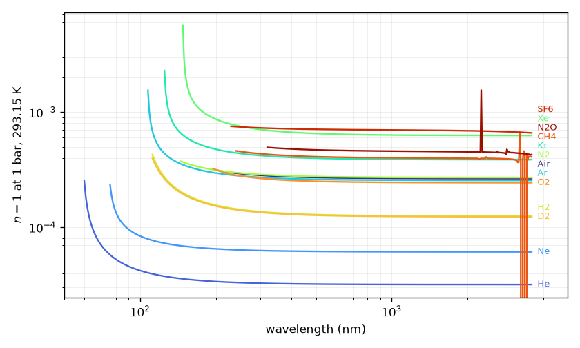
Refractivity of every gas at 1 bar and 293.15 K from optmat’s recommended models, each drawn from the shortest wavelength its model is qualified for to 3.6 µm (the infrared-active molecules’ qualified windows have gaps, drawn through here). A factor of twenty separates helium from xenon.

Density

density() returns the number density in m⁻³ from optmat’s real-gas equations of state (CoolProp’s Helmholtz-energy equations, through optmat.gas.eos), adapted by OptmatGas. pressure() inverts it exactly and ideal_gas_density() gives \(p/k_\mathrm{B}T\) for comparison.

Note

Pressures are in bar. This is the one documented departure from SI at the user interface (conventions, §1), because the field works in bar. Everything else is SI, and temperatures default to 293.15 K.

The equation of state is real-gas, which matters for the high-pressure fills used in self-compression: argon at 293.15 K departs from ideal by 0.14 % at 2 bar and 2.5 % at 40 bar. Below 0.1 bar every gas here is within 0.2 % of ideal, and below 1 mbar within 2 × 10⁻⁵. A pressure of exactly zero returns zero without consulting the equation of state, which is undefined there — a gradient fill terminating in vacuum needs that. A condensed state is refused (below).

Third-order nonlinearity

gamma3() is the per-particle hyperpolarisability in m⁵/V², so \(\chi^{(3)}\) is strictly linear in number density. It is optmat’s electronic Kerr coefficient evaluated at a carrier, so it needs one: gamma3("Ar", wavelength=800e-9) (the electronic Kerr coefficient at the carrier). chi3() and n2() need it too, as wavelength= or as the selection’s carrier_wavelength, and are refused without one. The nonlinear index follows from

\[n_2 = \frac{3\chi^{(3)}}{4\varepsilon_0 c\, n_0^2},\]

with \(n_0\) read at the same carrier; n2_from_chi3() and chi3_from_n2() are that relation and its inverse. One run takes one coefficient per species, at its carrier.

Air has no Kerr coefficient and raises; its nonlinearity comes from the nitrogen and oxygen of a mixture (mixtures).

Ionisation and Raman data

ionisation_potential() returns optmat’s first ionisation energy in joules for every gas but air. A built-in species carries it as IonisationData, a potential and its citation; the rate itself is optmat’s rate model (ionisation), and the energy the plasma loss pays is that model’s own.

A built-in gas’s Raman response is optmat’s (Raman responses from optmat), and a built-in species carries no Raman constants (raman=None). raman_status() reports what optmat holds for a gas: "validated" for N₂, O₂, H₂, D₂, CH₄ and SF₆, "provisional" for N₂O, and "atom" for the noble gases. prop_capillary and prop_waveguide turn the Raman response on by default for every validated molecule; for N₂O they leave it off and warn, except under MaterialSelection(raman="provisional"), which turns optmat’s provisional N₂O response on, with one status warning per run. A caller’s own molecular constants go on a custom species as a MolecularRaman, from solprop.physdata.raman_types (also exported by solprop.physdata), with each dephasing rate a Linewidth: a constant term, a Dicke-narrowing term and a collisional term, so a gas with only a measured \(\tau_2\) is the special case with the constant alone (Raman).

Silver and aluminium

silver() and aluminium() return optmat’s tables, table/Ag and table/Al (solids), for waveguide walls. A table carries its interpolant’s exact derivative. Outside the tabulated support the endpoint is held with a warning; that is not a physical extrapolation. For a good metal it is wrong in a known direction: \(n\) and \(k\) grow as \(\sqrt{\lambda}\) in the Hagen–Rubens regime, so a held endpoint understates both beyond the long-wave end. An optical grid does not reach there, but a terahertz grid on a metal wall would.

Window glasses

Five glasses join fused silica for the offline optics of the compression page: a window, a pair of wedges, a lens. glass() finds any of them by name, and each factory returns optmat’s recommended model (solids): calcium_fluoride() (CaF2), magnesium_fluoride() (MgF2), bk7() (BK7, N-BK7), sapphire() (sapphire, Al2O3) and barium_fluoride() (BaF2). Magnesium fluoride and sapphire are uniaxial and need a ray, axis="o" or axis="e". A caller’s own formula is a SellmeierGlass — a sum of poles with an analytic frequency derivative — or a TabulatedGlass, which warn outside their stated range as optmat’s models do.

Where solprop’s choices differ from Luna.jl’s, the differences are listed in Noteworthy differences from Luna.