Polarisation and azimuthal modes

This page is for anyone propagating more than one transverse field component: an elliptically or circularly polarised input, a pair of polarisation partners, or modes whose field direction varies across the cross-section (TE, TM and the higher-order HE modes). It covers the two ways the state can carry two components, the Jones and Stokes helpers and their sign conventions, the angular quadrature a vector mode set needs, how the plasma and Raman responses act on the synthesised Cartesian field, and the non-degenerate partners of a rectangular guide.

Where the polarisation is declared. The keyword drivers propagate one transverse component per mode row, and polarisation= on prop_capillary and prop_waveguide is refused by name. Polarisation enters through the mode set instead: pass modes= a set that holds both partners, or TE, TM and higher-order HE modes. with_polarisations() adds the orthogonal partner of every degenerate mode, mode.rotated(np.pi / 2) gives one by hand, and marcatili() builds a set of HE, TE and TM capillary modes. The keyword pulse then excites the first row only; an input spread over several rows, such as the elliptical launch below, is given as an explicit initial field to a Simulation or to solprop.translate.problem.assemble. A polarisation-resolved capillary run through the drivers is not validated end to end (the refusal of polarisation= says so). The free-space routes take a Jones vector on SpatialPulse (jones=), and a general modal guide can declare circular and split channel bases.

Amplitudes and fields

A modal input or saved amplitude is in square roots of watts. Its squared analytic amplitude integrates to true energy after summing modes and polarisation components. Broadband run statistics use the Hermitian Poynting trace described in power and intensity. Assembly divides the spectral amplitude by sqrt(Re n_eff) before the transverse mode functions synthesise Cartesian electric fields in V/m at the quadrature nodes. Those functions retain the internal vacuum normalisation (epsilon0*c/2) integral |e|**2 dA = 1.

Modal phases and local intensity

Modal powers alone do not determine the transverse intensity. The physical field is a coherent sum of the modal fields: changing their relative phase can move intensity across the core while leaving the energy in each mode unchanged. The RDW lesson plots modal energies; use a field reconstruction when the local spatial pattern is the quantity of interest.

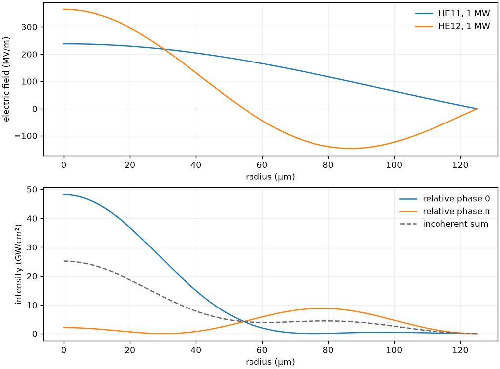
An illustrative coherent superposition in the index-one limit. Each of the two modes carries 1 MW in both cases, but their relative phase changes the local intensity. The dashed curve adds intensities without interference and therefore cannot represent either coherent field. Profiles are calculated from a 125 micrometre capillary; this is not a propagation result.

A coupling between runs keeps the polarisation as a Jones state in each plane’s own oriented frame; mirrors and Jones elements change the frame and the field together (coupling simulations).

Two equivalent representations

The state has shape (n_modes, n_pol, n_omega) before assembly adds its batch axis. There are two ways to represent the same vector field:

Representation	Mode set	State polarisation axis	Resolved components
Separate mode rows	Orthogonal, degenerate modes	n_pol=1	("x", "y")
Product with a common spatial profile	One scalar profile	n_pol=2	One component of that profile

The first representation also describes TE, TM and higher-order HE modes, whose Cartesian direction varies across the cross-section. The second is useful when x and y share one scalar spatial profile. The combined number of physical components is transform.n_pol * n_pol, at most two. A two-component state on a mode that itself requires x and y must therefore specify a valid single component explicitly.

Where both apply – an HE11 pair, uniformly polarised – they are the same run: the pair’s cross components are exact zeros, so the first adds only exact zeros to the second’s sums, and ten steps of a linearly and of a circularly polarised Kerr run on the reference backend agree bitwise (tests/backends/test_numpy_ref_multimode.py).

Omitted components are resolved from the union of the nonzero Cartesian components of the modes. An ordinary HE1m mode at phi=0 selects ("x",) (the unrotated capillary mode is the x-polarised, even member); its orthogonal partner at phi=pi/2 selects ("y",). Oblique HE1m, higher-order HE, TE and TM modes require both. A requested component that vanishes identically across the entire mode set is an error, with the modes and their angles in the message. An exact axis is classified analytically: a small nonzero angle is not rounded onto it. Custom mode implementations declare this property with Mode.principal_component(z), returning None for both.

Here is the same elliptically polarised input in the two representations. The Jones coefficients are specified in the optics convention and converted at the Fourier boundary:

import numpy as np
from solprop.fourier import to_internal
from solprop.grid import EnvelopeGrid
from solprop.modes import MarcatiliMode, transverse_quadrature
from solprop.polarisation import horizontal, rotate, waveplate
from solprop.pulses import GaussianPulse

grid = EnvelopeGrid.from_limits(0.002, 800e-9, (300e-9, 2e-6), 100e-15)
mode = MarcatiliMode(125e-6, cladding=1.45, loss=False)
pulse = GaussianPulse(wavelength=800e-9, fwhm=15e-15, energy=2e-6).build(grid)
jones = to_internal(rotate(waveplate(np.pi / 2), np.pi / 5) @ horizontal())
product_input = pulse * jones[None, :, None]
row_modes = [mode, mode.rotated(np.pi / 2)]  # x, then y
row_input = product_input.transpose(1, 0, 2).copy()
product_rule = transverse_quadrature([mode], n_r=24)
row_rule = transverse_quadrature(row_modes, n_r=24)

Pass the corresponding modes, input and quadrature to solprop.translate.problem.assemble; the solver and nonlinear response declarations are otherwise identical. When comparing the representations, use total energy and peak_power_total: individual mode powers label different pieces of the state. Fibre peak_intensity retains its definition as peak intensity on the waveguide axis.

Jones, Stokes and ellipse helpers

solprop.polarisation works in the optics convention with Jones order [E_x, E_y]. It supplies a horizontal unit vector, an ideal horizontal polariser, a waveplate, passive coordinate rotations and rotated optical elements. A waveplate’s fast axis is x: a positive retardance delays the y component relative to x, a positive phase in the optics convention, so a quarter-wave plate turns light linear at +45° into (x + i y)/sqrt(2). The Stokes definition is

\[I=|E_x|^2+|E_y|^2,\quad Q=|E_x|^2-|E_y|^2,\quad U=2\operatorname{Re}(E_x E_y^*),\quad V=-2\operatorname{Im}(E_x E_y^*).\]

Thus (x+i*y)/sqrt(2) has positive V, and its conjugate has negative V. This algebraic sign avoids a viewing-direction ambiguity in the words right and left circular. Where the package does have to say those words — a guide’s circular channel labels — it says them once, in solprop.modes.guide.circular_pair(), against this sign: positive \(V\) is left, and Circular and coupled modal bases derives it. stokes(..., normalise=True) requires nonzero intensity. cartesian returns the three normalised Poincaré coordinates. Stokes inputs must be real and finite, with I >= hypot(Q,U,V) up to the documented arithmetic rounding at the cone surface.

The ellipse semiaxes are sqrt((I+L)/2) and sqrt((I-L)/2), where L=hypot(Q,U); the orientation of the major axis from x is atan2(U,Q)/2. The ellipticity is the minor-to-major ratio. Linear light has ellipticity zero and circular light one. Circular and zero fields have zero orientation by convention; the ellipticity of zero light is undefined and raises PolarisationError. For partially polarised input these are the equivalent ellipse parameters, not a claim that the field has a single deterministic Jones vector. These helpers act on Jones vectors and Stokes parameters you supply; no ellipticity statistic is recorded during propagation.

Angular integration and plasma

ModeCollection.marcatili(radius, gas, pressure, kinds, n, m) builds an ordered set of hybrid ("HE") and transverse ("TE", "TM") capillary modes, one per entry of the three sequences, which must have the same length; with_polarisations() then adds the degenerate orthogonal partners. The transverse quadrature must resolve their angular dependence. The Cartesian harmonic of HE modes is h=abs(n-1); TE and TM have h=1. A Kerr projection contains four modal factors, so the periodic angular rule must integrate degree 4*h. The sufficient condition is n_theta >= 4*h+1.

In an isotropic medium HE11 can populate HE12 but cannot populate HE21, and TM01 cannot populate HE11. Too few angular nodes break these selection rules. With two nodes for an HE11/HE31 set, for example, the harmonic-two function aliases to a constant and the projection populates a forbidden mode; the quadrature constructor warns when n_theta is below 4*h+1 for the modes it is given.

On a field grid, vector plasma takes its ionisation rate from hypot(E_x,E_y) and directs the ionisation-loss current along the field. Independently of its direction, E dot J_loss = rho * Ip * W * (1-f), so time-integrated loss is rho * Ip * (f_final-f_initial) per unit volume. A circular Gaussian test subtracts helium and argon with one analytic rate, cancelling their common Drude current; the spectral energy derivative must pay precisely the difference of their ionisation potentials times the generated electrons. The error bound integrates the second derivative of the Gaussian loss current for the prefix trapezoid, adds rounding and the pulse tails, and is declared before measurement. Three temporal resolutions must show second-order convergence. Vector Raman acts on the same synthesised Cartesian field using explicitly labelled isotropic and rank-two histories. Both real-basis representations, higher HE and TE/TM modes are supported; see the standalone Raman treatment for delayed coherence, circular limits and the scalar-only refusal for undeclared custom tensors and silica.

On an envelope grid, EnvelopePlasmaResponse averages the instantaneous rate around the local polarisation ellipse. Both modal representations above produce the same Cartesian ellipse at each spatial node. Its two independent loss moments determine the vector current: an intermediate ellipse generally loses different fractions of its major- and minor-axis amplitudes. Multiplying the envelope by a single scalar loss coefficient gives the wrong direction even if the total work agrees. The zero-field, linear and circular limits are continuous. The envelope plasma sources give the rate convention, source units and frequency factors. The detailed plasma chapter derives the two moments and gives an analytic example in which a scalar loss coefficient matches the work but misses the current by 18.35%.

Rectangular polarisation partners

A rectangular guide’s x and y partners are not generally degenerate. Supply both as separate mode rows, for example ModeCollection.with_polarisations([RectMode(a, b, ...)]), and give each row one state component. Simulation.from_waveguide infers the required physical components from that set. Its shaped input excites the first row; use direct Simulation construction with a field for each row to launch both. Each row then receives its own linear operator. The shared spatial-profile, two-component layout is refused for RectMode because it would duplicate one partner’s index.