Coherent capillary walls#

Use a coherent wall when relative modal phases affect leakage and coupling at a capillary boundary. Begin with the practical capillary workflow, then use the equations and validity ratios here to assess the approximation. Ordinary independent modal loss is described in Capillary modes and dispersion.

The coherent wall#

Marcatili’s loss is incoherent: each \(\mathrm{HE}_{1m}\) channel attenuates on its own and the wall never moves power between them. That is right whenever the channels are far apart in propagation constant compared with the wall’s coupling, and wrong whenever they are not — two channels that graze the same lossy boundary exchange amplitude with a definite phase, and an aperture or a taper that fills several of them at once can see that exchange before it sees the attenuation.

prop_capillary(..., modes=N, wall=CoherentWall()) propagates the coherent wall instead. Use it when several \(\mathrm{HE}_{1m}\) modes are excited together — a launch that is not matched to \(\mathrm{HE}_{11}\), an aperture, a taper — and the exchange between them matters; a run in which only \(\mathrm{HE}_{11}\) matters gains nothing from it. The block condenses the outgoing Robin boundary condition of the exact radial problem onto the \(N\) retained channels. That boundary condition, and the observation that an incoherent modal loss misjudges the loss of beams that pull away from the wall, are Andreasen and Kolesik’s semitransparent wall (Phys. Rev. E 87, 053303 (2013), Eqs. 10–15; J. Lightwave Technol. 31, 2999 (2013)), which they apply on a finite-difference grid; the condensation onto modes is solprop’s own. It makes the wall one rank-one term that couples every channel to every other:

\[G = D + H,\qquad D = -\frac{i}{2ka^2}\operatorname{diag}(u_m^2),\qquad H = g(a)\,hh^{T},\]

with \(h_m = -\sqrt2\,\operatorname{sgn}J_1(u_m)\,u_m\) — the radial derivative of the \(m\)-th orthonormal basis function \(\phi_m(x)=\sqrt2\,J_0(u_mx)/|J_1(u_m)|\) at the wall — and \(g(a) = i/[2ka^2(2N - ik_{\rm eff}a)]\), with \(N\) the number of retained channels. The carrier \(k = n_{\rm core}\omega/c\) is the in-core wavenumber the paraxial reduction divides by; the impedance \(k_{\rm eff} = k_0/v_n\) is the vacuum wavenumber \(k_0 = \omega/c\) over the same cladding term \(v_n = (\varepsilon+1)/(2\sqrt{\varepsilon-1})\) the ordinary Marcatili index already uses, which is the combination whose \(N = 1\) limit reproduces it.

It reproduces Marcatili’s loss to a bound you can write down. With \(t = v_n/(k_0a)\), the condensed diagonal’s imaginary part is \(-2u_m^2t/(1 + 4N^2t^2)\) against Marcatili’s \(-2u_m^2t\), and the paraxial reduction divides by \(2k\) where the exact square root divides by \(2\,\mathrm{Re}\,\beta\), so each channel’s field-loss rate departs from \((\omega/c)\,\mathrm{Im}\,n_{\rm eff}\) by

\[-\left(4N^2t^2 + \frac{u_m^2}{2(ka)^2}\right)\]

relative. For a 125 µm bore at 800 nm with one channel that is \(-1.2036\times10^{-5}\), and that is what is measured. The first term is the square of the quasi-static ratio \(2N/|ak_{\rm eff}|\) the block records as a validity limit, which is the reason raising \(N\) cannot by itself improve the condensation: the boundary trace it discards grows with the basis.

The subsections below give the block’s requirements and validity limits, its effect on a straight bore, how it is integrated and recorded, and its extension to a taper or a pressure gradient. Separate chapters describe taper coupling without a wall and the vector wall, which gives TE and TM fields their own impedances. The capillary chapter of the guide sets out when and how to use it.

What it needs, and what it refuses#

The condensation is onto the complete set of \(J_0\) radial orders, so the block needs the contiguous set \(\mathrm{HE}_{11}\) to \(\mathrm{HE}_{1N}\) — modes=N on the capillary route builds exactly that — sharing one polarisation angle, one capillary model and one declared guide. A sparse set, a mixed family, two polarisations, a noise model and a fused batch are refused by name, each at the layer that owns the refusal. All three backends execute the block — numpy_ref, numba_cpu and native, on the CPU and on the qualified GPU builds (the native backend) — except that method="cf4" runs on numpy_ref alone. The vector boundary response chapter covers the additional families and is declared instead of it rather than beside it.

Two settings are refused rather than quietly overridden, because the block is what they describe. The wall is the loss model: it replaces each channel’s Marcatili attenuation, so loss= must be True — False, a scale or a measured curve beside a wall would otherwise vanish without a word, and is refused by name instead. And the condensation inverts the full model’s transverse eigenvalue, so model="reduced" is refused too. A tube lattice is refused for the same kind of reason: an antiresonant guide’s loss is its tubes’ resonances, not a Robin condition at one radius, so lattice= and wall= together are named rather than given the bare capillary’s wall.

Validity ratios. Three dimensionless ratios, taken for the highest retained channel, say how far the block is from its assumptions:

\(u_N/(ka)\), how far that channel is from paraxial;
\(u_N/(k_0a)\), the grazing ratio the Marcatili expansion is asymptotic in;
\(2N/|ak_{\rm eff}|\), the quasi-static ratio above.

They are computed over the scored band — the run’s grid.inband_mask, the requested wavelength limits the step’s error norm measures — and recorded on the run’s identity. Above validity_limit (default 0.25) the block is refused, and above a tenth of it the construction warns, naming the ratio. The operator itself is built over the wider active band (grid.active_mask), whose spectral collar reaches half the lowest requested frequency; the collar is absorbed and not scored, so its bins, where every ratio would be about twice its in-band value, neither refuse nor warn. A grid whose requested limits hold no bin takes the ratios over the whole active band instead. Bins outside the active band are never evaluated: the formula divides by \(\omega\), and the generator is left exactly zero there.

On a straight bore#

Here is the whole of it, on ten steps of a 50 µm bore, against the same run with the wall left off. Both launch into \(\mathrm{HE}_{11}\) alone; what appears in the other two channels is the wall’s doing, because a diagonal loss cannot move power between channels at all and the only other path — the Kerr overlap — is eleven orders below it.

import warnings

import matplotlib.pyplot as plt
import numpy as np

from solprop.boundaries import absorber
from solprop.driver import prop_capillary
from solprop.grid import FieldGrid
from solprop.modes import CoherentWall
from solprop.stepper import FixedSchedule

length, steps = 2e-4, 10
grid = FieldGrid.from_limits(length, 800e-9, (400e-9, 1.6e-6), 300e-15)
schedule = FixedSchedule(np.full(steps, length / steps))

def run(wall):
    # The band runs past helium's and silica's fitted ranges and a fifth of a
    # millimetre of this bore is a marginal geometry on purpose, so both say so.
    with warnings.catch_warnings():
        warnings.simplefilter("ignore")
        return prop_capillary(
            50e-6, length, "He", 1.0, lambda0=800e-9, grid=grid,
            # A collar weak enough that twenty-micrometre steps are stable: an
            # absorber is an explicit term in the nonlinear scheme.
            absorber=absorber(grid, boundary_length=1e3),
            fwhm=30e-15, energy=1e-9, modes=3, n_save=6,
            backend="numpy_ref", wall=wall, schedule=schedule,
            dz_max=length / steps, dz_init=length / steps,
            plasma=False, raman=False,
        )

walled, plain = run(CoherentWall()), run(None)
print(walled.metadata.modal["flow"]["quasi_static"])

fig, ax = plt.subplots(figsize=(6.4, 3.8))
for handler, style, label in ((plain, ":", "wall=None"), (walled, "-", "CoherentWall()")):
    planes = handler.planes()
    z = np.array([plane.z for plane in planes]) * 1e6
    energy = np.array(
        [np.asarray(plane.stats["energy"]).reshape(3, -1)[:, 0] for plane in planes]
    )
    for channel in range(3):
        ax.semilogy(
            z, energy[:, channel] / energy[0, 0], style, color=f"C{channel}",
            label=f"HE_1{channel + 1}, {label}",
        )
ax.set_xlabel("z (um)")
ax.set_ylabel("fraction of the launched energy")
ax.set_ylim(1e-22, 3.0)
ax.legend(frameon=False, fontsize="small", ncol=2)
fig.tight_layout()

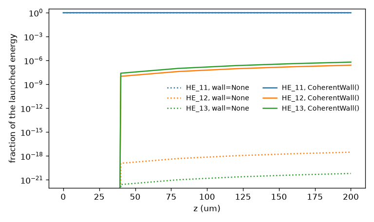
../../_images/modes-coherent-wall.png — The coherent wall moves power between channels; the incoherent one cannot. Ten fixed steps of 20 micrometres of a 50 micrometre helium-filled bore, launched into HE_11 alone, with the fraction of the launched energy found in each channel at each save plane. The uncoupled route leaves 1e-18 and 1e-21 in the upper channels – the capillary’s Kerr overlap, and nothing else.#

How it is propagated#

The block is a coupled flow, so it cannot ride the cumulative diagonal operator the rest of the package uses. The run is split instead: the shared scalar part of the flow — the first channel’s own operator, in the one co-moving frame — stays in the cumulative \(\Phi\), where it is integrated analytically and commutes with everything, and the modal part becomes the linear.coupled_flow leaf of the kernel contract. Nothing may be split between them that does not commute, and a channel-dependent diagonal does not, which is why \(\Phi\) is built over \(N\) copies of one channel and carries no mode dependence at all. The per-channel true-power weight is unaffected: it is a row of its own, and a saved amplitude still carries each channel’s \(\sqrt{\mathrm{Re}\,n_{\rm eff}}\).

What the split leaves on the flow’s diagonal is \(k-\beta_{11}\), the block’s in-core carrier \(k = n_{\rm core}\,\omega/c\) less the first channel’s propagation constant. The two wavenumbers agree to five or six digits, so their difference would carry the absolute rounding of \(k\), about \(5\times10^{-9}\) 1/m and up to \(5\times10^{-10}\) of the difference itself; it is formed instead from the two refractivities, \(\big((n_{\rm core}-1)-(n_{\rm eff}-1)\big)\,\omega/c\) (core_index_minus_one(), neff_minus_one()), which is exact to \(10^{-14}\) of itself. On a guide that varies along z this is what lets each section’s expansion resolve to its \(10^{-12}\) target (SECTION_TOL): forced to degree 64, the qualification tapers’ generators floor at \(4\times10^{-14}\), so a section still unresolved at the highest degree is refused, never accepted with a larger error.

The reference backend integrates the section with a Schur matrix-function action, \(U = Z\exp(\Delta z\,T)Z^{\rm H}\), once per stage fraction, and takes the inverse the interaction picture needs as the matrix function of the negated exponent rather than as a solve. Because the geometry is constant there is no explicit residual at all, and the certificate the leaf carries — the Schur reconstruction residual and unitary defect amplified by the departure from normality, and a bound \(\exp(\Delta z_{\max}(\mu_{\max}-\mu_{\min}))\) on \(\|U\|\,\|U^{-1}\|\) — is checked against the measured action at every step rather than trusted. A step whose \(\|U\|\,\|U^{-1}\|\) exceeds condition_limit (default \(10^4\), about nine e-foldings of attenuation of the lossiest retained channel in one step) is refused, because the inverse action carries the interaction-picture source back and an unbounded inverse would amplify it. Over ten steps the coupled route costs about 1.4 times the uncoupled one for a single channel and about 1.8 times for eight.

wall_square_root_metric() builds the square-root model \(c' = iBc\) and its candidate flux metric \(W = (B+B^{\rm H})/2k\) as a diagnostic. Its identity \(d(c^{\rm H}Wc)/dz = -c^{\rm H}(M-M^{\rm H})c/2ik\) is exact algebra for a constant real positive carrier and that is the whole of its domain: it does not establish positivity of \(W\), and what a run propagates is the paraxial generator above, not the square root.

Reading the record#

A run carrying a wall writes a flow entry on its modal identity, so what the block was is recoverable from the file alone: output.metadata.modal["flow"] is a mapping of the section method, the two identity strings, the core radius, the three validity ratios and the three certificate rows reduced to their extremes, every one of them a scalar or a string so that it can be part of the key a resume is checked against. Four entries describe the sectioning itself:

entry	what it says
`n_sections`	how many frozen sections the run was cut into — the operator table’s own intervals times `CoherentWall.sections`. `1` for a constant bore
`n_deg`	the Chebyshev degree along z the generator resolved at, plus one. `1` for a constant bore, which is one coefficient and no z dependence; 17 on the taper below
`connection`	whether the flow carries the HE1m connection \(C\), which is `True` exactly when the radius varies. A pressure gradient in a fixed bore carries none
`advisory_step`	\(0.9/(K\,\|U\|\|U^{-1}\|)\) in m, the smallest over every section and every frequency the error norm scores (the residual is applied nowhere else), which is what a declared step is warned against. Infinite for a flow with an exactly zero residual

The geometry the record names — the radius and the three ratios — is the worst the run reaches, scanned over every section edge and midpoint, not the entrance’s, so a resume across a changed taper is refused by the field that moved.

Printing the record shows the same thing on one flow row, which reads diagonal for every run that carries no block and, for one that does, mean impedance coherent wall, constant_schur, worst ratio 4.491e-02, conditioning 1.007e+00, or, for the taper below, mean impedance coherent wall, frozen_residual, frozen_residual, frozen_residual, frozen_residual, worst ratio 5.613e-02, conditioning 1.013e+00. The run’s capability is that of any modal run — a coupled flow through a basis does not change the basis — so every ordinary modal accessor is admitted on such a file.

The worked examples run the wall over metres: a pressure-gradient compressor, a tapered capillary and the vector wall. The coherent wall of a capillary, against the incoherent one runs this section end to end: the loss limit against its derived departure over a band of wavelengths, and the conversion against the incoherent route. The same linear.coupled_flow leaf is what a declared basis of a split block becomes on the general modal route (general modal propagation).

A guide that varies along z#

A taper or a pressure gradient is carried too; a taper without a wall carries the same connection (the taper coupling without a wall). The run is cut into sections — the linear operator’s own intervals, which already land on every declared corner of the radius and the fill, subdivided sections times — and inside each one the complete generator is frozen at the midpoint and integrated by the Schur matrix-function action a constant bore uses (above). What the freezing leaves out is put back exactly, as an explicit term in the Runge-Kutta source:

\[R_s(z) = D(z) - D(z_s) + H(z) - H(z_s) - C(z).\]

The connection. The last piece of \(R_s\) is the connection \(C\). The basis is attached to the core radius, so a taper moves it, and writing the field in the local basis at every \(z\) costs

\[C_{mn} = \frac{a'}{a}\,\frac{2s_ms_nu_mu_n}{u_m^2-u_n^2}\quad(m\ne n), \qquad C_{nn} = 0,\]

with \(s_m = \operatorname{sgn}J_1(u_m)\), which is \(\langle\psi_m|\partial_z\psi_n\rangle\) for \(\psi_n = \sqrt2J_0(u_nr/a)/(a|J_1(u_n)|)\) and is checked that way, by differentiating the profile the run actually declared rather than by trusting the formula. It is real and antisymmetric in the true-power amplitude \(b_n = \sqrt{w_n}\,a_n\), where coupled local-mode theory puts it, so the kernel stores \(\sqrt{w_n/w_m}\,C_{mn}\) for its own amplitude and on its own it moves no power out of the retained set at all; what it does is convert the launch between the channels, and the channels it converts into are the lossier ones. That, and not a larger attenuation at a smaller radius, is what a non-adiabatic taper costs: a 50 to 40 µm transition over a fifth of a millimetre leaves 3.8 % of the energy in \(\mathrm{HE}_{12}\) and 3.3 % in \(\mathrm{HE}_{13}\), and loses 1.9e-3 of it where the adiabatic route (taper_coupling=False), which cannot convert at all, loses 6.4e-4.

Why the wall block is not re-weighted. The wall block’s own off-diagonal is not stored with the \(\sqrt{w_n/w_m}\) weights, and the difference is physics rather than convention: the condensed \(M = k^2I + L_N/a^2\) is the matrix of a reciprocal operator in a real orthonormal basis, so it and every function of it — the exact one-way generator \(i(\sqrt{M}-k)\) included, whatever the loss — are complex symmetric in the field amplitude, and the diagonal \(W^{\pm1/2}\) would break that symmetry. The re-weighting would change the off-diagonal by \((w_m-w_n)/(2w)\) of itself, 0.17 1/m of 148 at 3.2 µm on a 50 µm bore, which is 2.4 times smaller than the paraxial reduction’s own symmetric departure from the exact square root: below the model’s approximation, and in the wrong symmetry class.

Freezing is exact. Because \(R_s\) is evaluated exactly, freezing is a rearrangement of the same equation and not an approximation: one frozen block per interval and four of them give answers 1.85e-10 apart on that case. What sections buys is a smaller explicit term, and the flow records the bound on it, together with the advisory step \(0.9/(K\,\|U\|\|U^{-1}\|)\), with \(K\) the bound on the norm of the explicit term, \(\|U\|\|U^{-1}\|\) the conditioning of the frozen section’s propagator, and 0.9 a margin below the Runge-Kutta scheme’s stability radius on the imaginary axis. A declared dz_init, dz_max or fixed schedule above that limit is warned about by name, with the term, the section, the frequency and the numbers, and nothing is changed behind your back. The limit is advisory, but a fixed schedule several times above it on a long taper can go unstable, so heed the warning.

The residual acts only where the error norm looks. It is applied on the bins the adaptive error norm scores, the requested wavelength band (inband_mask), and not in the spectral collar around it, where the wall block is still evaluated but the controller never looks. The residual can be largest there — 7.2e3 1/m at 5.85 µm at the end of a 20 cm section of a 100 to 60 µm taper, against 3.8e3 in band — and at the steps the in-band error allows, |R| dz of about 4, the embedded Runge-Kutta pair would be unstable on it with nothing to see the growth (it would show as a spurious HE_14 transient near the taper’s corner). In the collar the frozen flow alone carries the state, exact at any step: each section’s midpoint block, without the variation across the section and without the taper connection. There freezing is an approximation, but one no result depends on. The flow is diagonal in frequency and the controller and the hard mask act per bin, so an in-band bin reads the collar only through the nonlinear source and the temporal absorber, and the in-band answer moves by at most the product of that coupling, the dropped term and the collar’s share of the field: below 1e-18 of the in-band field on the tapers tested, with a measured effect of 6e-20.

Every channel keeps its own normalisation. The cumulative \(\Phi\) must be a multiple of the identity in the channel axis, so the term that renormalises a vacuum amplitude along a varying index, \(-\tfrac12\ln[w(z)/w(0)]\) with \(w = \operatorname{Re} n_\text{eff}\), is the lowest channel’s there. The rest of each channel’s own is carried in the flow’s diagonal, beside the block:

\[-\tfrac12\,\frac{d}{dz}\ln\frac{w_n}{w_1} = -\tfrac12\left(\frac{w_n'}{w_n} - \frac{w_1'}{w_1}\right),\]

real, zero for \(\mathrm{HE}_{11}\) and zero wherever the guide does not vary, with the slope \(w_n' = \operatorname{Re}\,dn_\text{eff}/dz\) taken in closed form through the radius and the fill (dneff_dz()), never by a difference. It is part of the generator, so the frozen block, the explicit residual and CF4 all carry it. On the 50 to 40 µm taper below, leaving it out — giving every channel the lowest channel’s normalisation — moves \(\mathrm{HE}_{12}\) and \(\mathrm{HE}_{13}\) relative to \(\mathrm{HE}_{11}\) by \(9\times10^{-6}\) and \(3\times10^{-5}\) at 800 nm and by \(1.5\times10^{-4}\) and \(5.5\times10^{-4}\) at the edge of the active band; with it they agree with an independent solve in the true-power amplitude, which has no normalisation term at all, to the step error: \(1.5\times10^{-8}\) at ten steps, falling at fifth order. The passivity guard of the varying route allows each channel its own term, and nothing more.

What the profile and the schedule must do. The profile must have an analytic derivative — a FromCallable without a slope is refused, because a difference of samples is noise and not a slope — and every channel must declare the same radius and density profiles, compared by their structural identity rather than by their value at the entrance, so that two tapers agreeing only at \(z = 0\) are named instead of silently propagating the first one.

A fixed schedule must land on every corner of the profile exactly. The sections are placed on those corners, and the section a stage reads is matched to a tolerance of \(10^{-10}\) of the run; a schedule edge that comes near a corner without landing on it anchors its step on the closing side and then integrates past the corner against a frozen block its own stages do not read, which costs the run its order. Such a schedule is refused by name; FixedSchedule.uniform lands on every corner, and adaptive stepping needs no rule at all, because the driver lands on the hard kinks itself.

A taper, measured. Here is a taper with the wall, on the same ten steps as the straight bore, against the adiabatic route (taper_coupling=False, no wall). The launch is into \(\mathrm{HE}_{11}\) alone in both, so everything in the upper two channels is the connection’s doing: the uncoupled route leaves \(10^{-18}\) there and a walled straight bore \(10^{-6}\).

import warnings

import matplotlib.pyplot as plt
import numpy as np

from solprop.boundaries import absorber
from solprop.driver import prop_capillary
from solprop.grid import FieldGrid
from solprop.modes import CoherentWall
from solprop.profiles import PiecewiseLinear
from solprop.stepper import FixedSchedule

length, steps = 2e-4, 10
# Straight, transition, straight, at a radius and length ten fixed steps resolve.
taper = PiecewiseLinear.from_stages(
    (0.0, 6e-5, 1.4e-4, 2e-4), [50e-6, 50e-6, 40e-6, 40e-6]
)
grid = FieldGrid.from_limits(length, 800e-9, (400e-9, 1.6e-6), 300e-15)
schedule = FixedSchedule(np.full(steps, length / steps))

def run(wall):
    # The band runs past helium's and silica's fitted ranges and this is a
    # marginal geometry on purpose, so both say so. The comparison drawn is the
    # adiabatic route, the declared opt-out taper_coupling=False.
    with warnings.catch_warnings():
        warnings.simplefilter("ignore")
        return prop_capillary(
            taper, length, "He", 1.0, lambda0=800e-9, grid=grid,
            # A collar weak enough that twenty-micrometre steps are stable: an
            # absorber is an explicit term in the nonlinear scheme.
            absorber=absorber(grid, boundary_length=1e3),
            fwhm=30e-15, energy=1e-9, modes=3, n_save=6,
            backend="numpy_ref", wall=wall, schedule=schedule,
            dz_max=length / steps, dz_init=length / steps,
            plasma=False, raman=False, taper_coupling=wall is not None,
        )

walled, plain = run(CoherentWall()), run(None)
record = walled.metadata.modal["flow"]
print(record["n_sections"], record["n_deg"], record["connection"])

fig, ax = plt.subplots(figsize=(6.4, 3.8))
for handler, style, label in ((plain, ":", "adiabatic"), (walled, "-", "CoherentWall()")):
    planes = handler.planes()
    z = np.array([plane.z for plane in planes]) * 1e6
    energy = np.array(
        [np.asarray(plane.stats["energy"]).reshape(3, -1)[:, 0] for plane in planes]
    )
    for channel in range(3):
        ax.semilogy(
            z, energy[:, channel] / energy[0, 0], style, color=f"C{channel}",
            label=f"HE_1{channel + 1}, {label}",
        )
ax.set_xlabel("z (um)")
ax.set_ylabel("fraction of the launched energy")
ax.set_ylim(1e-22, 3.0)
ax.legend(frameon=False, fontsize="small", ncol=2)
fig.tight_layout()

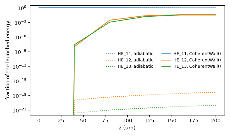
../../_images/modes-coherent-wall-taper.png — A taper converts between channels, and the conversion is what it costs. Ten fixed steps of 20 micrometres of a helium-filled bore running 50 micrometres, tapering to 40 over 80 micrometres and holding, launched into HE_11 alone, with the fraction of the launched energy in each channel at each save plane. The walled taper loses 1.9e-3 of the launched energy where the uncoupled one loses 6.4e-4, and the difference is the 7 % converted into the lossier orders.#

Mode conversion and loss in a taper with a coherent wall runs this taper beside the two straight bores it joins, reads the sectioning off the record, and shows that four frozen sections per interval and one give the same answer to \(2\times10^{-10}\).

Integrating the varying section by CF4. CoherentWall(method="cf4") integrates each section’s whole generator by the fourth-order commutator-free exponential instead of freezing it: no explicit residual, so no advisory step, but a flow error the step controller cannot see and a run that is at most fourth order. It is admitted only where its internal factors provably cannot exceed \(\exp(h\,m_{\rm hi})\) — the largest norm the exact flow could have over a step \(h\), with \(m_{\rm hi}\) the largest eigenvalue of the generator’s Hermitian part — by more than growth_limit (default 2); a rejected section is refused by name, or integrated by the frozen split where fallback="frozen_residual" says so. That guard bounds growth, not accuracy: a lossless section passes it at any step, and only the step-doubling defect estimate, on which validate warns against rtol, says whether a step is small enough. On every taper measured a CF4 step costs 3.3 times a frozen one and is the more accurate only for steps beyond the frozen split’s advisory limit, so the default frozen split is the better choice at equal cost. CF4 is refused on a guide that does not vary, whose one section the constant-Schur action already integrates exactly; beside impedance="te_tm" it is admitted, because it integrates the stored expansion and reads nothing of the block that built it — measured fourth order, 3.996 and 3.999, on the vector taper below.