Radially and azimuthally polarised pulses: the vector wall over a metre

The launches here are pure capillary modes: linearly polarised HE_11, radially polarised TM_01 and azimuthally polarised TE_01. The latter two have cylindrical components independent of azimuth, but their Cartesian field directions rotate around the axis. A laboratory polarisation converter need not launch a pure radial mode. The two selected transverse families have the same core field shape, the same propagation constant to a part in \(10^9\), and the same nonlinearity – and they do not see the same wall. At grazing incidence the glass imposes one condition on the field tangential to it (TE) and another on the field normal to it (TM), and the TM field loses \(\varepsilon = n_{\rm glass}^2\) times faster. The scalar coherent wall gives the glass one averaged impedance; CoherentWall(impedance="te_tm") gives each field its own (Vector boundary response).

This example uses that vector wall in three ways:

1. the linear loss of the four lowest families across the band, from the wall block alone, against this package’s Marcatili formula and against what an impedance-averaged wall would give;

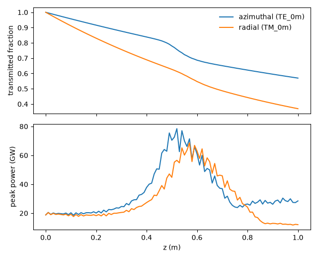
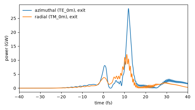
2. a 15 fs, 300 uJ pulse self-compressing through a metre of a 100 um bore filled with 3 bar of helium, launched once azimuthally (TE_0m) and once radially (TM_0m) polarised, three radial orders each;

3. the same pulse linearly polarised in HE_11, with the order’s second radial family EH_1m retained, where the wall’s anisotropy – the part the scalar average discards – converts HE_11 into EH_11.

What to look for. The two polarisations have the same leading core nonlinearity and nearly equal dispersion; their main difference here is the wall, where the radially polarised field loses energy about \(\varepsilon\) times faster. Both still self-compress, to a peak power of several tens of gigawatts a little past the middle of the metre, the radially polarised one somewhat lower; at the exit it carries about two thirds of the azimuthally polarised pulse’s energy. The duration printed at each peak is the width of a sub-cycle spike – the band reaches into the vacuum ultraviolet – not of a compressed envelope. The Kerr overlap also moves between a few parts in \(10^3\) and about a per cent of the energy into the higher radial orders. Both runs synthesise the full transverse field, E_x and E_y, for the Kerr term; a Kerr overlap formed from E_x alone would retain only the angular factor 3/8 of the full transverse-vector overlap, changing the model. Both components are therefore needed even though only one radial family is launched. In the HE_11 run the wall puts a few parts in \(10^7\) of the launch into EH_11 within the first ten centimetres, where the uncoupled run leaves \(10^{-34}\); it stays at that level, because HE_11 and EH_11 have different propagation constants and the exchange oscillates rather than accumulates.

What is approximate. The wall is the quasi-static, paraxial condensation of a grazing-impedance boundary, checked against the exact vector Maxwell roots family by family and through the coupled eigenvalue; it has not yet been checked against a resolved-cladding Maxwell solve excited in a mixed-family state. The gas index is optmat’s helium fit, qualified over the whole band (from 60 nm).

Each family’s own loss, across the band

One channel of each family in a 100 um bore, the vector wall block evaluated on its own with vector_wall_operator() – no run – against the Marcatili attenuation of the same channel. A negative azimuthal index is this package’s spelling of the EH family. The “impedance-averaged” curve is what a wall with one impedance gives the transverse families: the hybrid cladding term in place of each one’s own, which puts TE_01 and TM_01 on one curve.

import time
import warnings

import matplotlib.pyplot as plt
import numpy as np

from solprop.constants import C
from solprop.driver import prop_capillary
from solprop.exceptions import (
    GrazingIncidenceWarning,
    SolpropWarning,
)
from solprop.modes import CoherentWall, MarcatiliMode, vector_wall_operator
from solprop.processing import energy, fwhm_t, get_power
from solprop.processing import peak_power as peak_power_of

RADIUS = 100e-6
"""Core radius, m."""

LENGTH = 1.0
"""Capillary length, m."""

PRESSURE = 3.0
"""Helium pressure, bar."""

PUMP = {"lambda0": 800e-9, "fwhm": 15e-15, "energy": 300e-6}
"""The pump: wavelength (m), duration (s) and energy (J)."""

started = time.perf_counter()

wavelength = np.linspace(300e-9, 2e-6, 120)
omega = 2.0 * np.pi * C / wavelength
families = {
    "HE_11": ("HE", 1),
    "EH_11": ("HE", -1),
    "TE_01": ("TE", 0),
    "TM_01": ("TM", 0),
}


def channel(kind, order, radial=1, **fill):
    """Return one Marcatili channel of the bore, evacuated unless a fill is given."""
    gas = fill.get("gas")
    pressure = fill.get("pressure", 0.0)
    return MarcatiliMode(RADIUS, gas, pressure, kind=kind, n=order, m=radial)


def cladding_term(kind, order):
    """Return this package's Marcatili cladding term for one family, per bin."""
    return channel(kind, order).sampled_terms(omega).cladding_term


hybrid = cladding_term("HE", 1)
fig, ax = plt.subplots(figsize=(6.4, 3.8))
for index, (name, (kind, order)) in enumerate(families.items()):
    mode = channel(kind, order)
    block = vector_wall_operator([mode], omega, validity_limit=2.0)
    wall_rate = -np.real(block.generator[0, 0, :]) * 2.0
    marcatili = 2.0 * np.imag(mode.neff(omega)) * omega / C
    ax.plot(
        wavelength * 1e9, wall_rate, color=f"C{index}", label=f"{name}, vector wall"
    )
    ax.plot(wavelength * 1e9, marcatili, ":", color="k", linewidth=0.8)
    if kind in ("TE", "TM"):
        averaged = marcatili * np.real(hybrid) / np.real(cladding_term(kind, order))
        ax.plot(
            wavelength * 1e9,
            averaged,
            "--",
            color=f"C{index}",
            linewidth=0.8,
            label=f"{name}, impedance averaged" if kind == "TE" else None,
        )
ax.set_xlabel("wavelength (nm)")
ax.set_ylabel("power loss (1/m)")
ax.set_title("100 um bore: vector wall (solid), Marcatili (dotted)")
ax.legend(frameon=False, fontsize="small")
fig.tight_layout()

at_800 = int(np.argmin(np.abs(wavelength - 800e-9)))
for name, (kind, order) in families.items():
    block = vector_wall_operator([channel(kind, order)], omega, validity_limit=2.0)
    rate = -2.0 * float(np.real(block.generator[0, 0, at_800]))
    print(f"{name}: {rate:.4f} 1/m at {wavelength[at_800] * 1e9:.0f} nm")

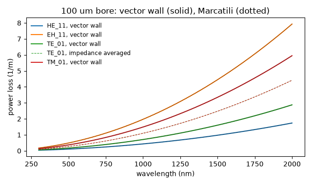
HE_11: 0.2766 1/m at 800 nm
EH_11: 1.2615 1/m at 800 nm
TE_01: 0.4512 1/m at 800 nm
TM_01: 0.9534 1/m at 800 nm

Radial against azimuthal polarisation

Each family retained with its first three radial orders – TE_01 to TE_03, and TM_01 to TM_03 – which is a set the vector wall accepts on its own. The pulse enters the first channel of the set. TE_0m and TM_0m do not couple through the wall (the nu = 0 block is diagonal in the two families), so the two families are two independent runs rather than one.

def propagate(modes, wall):
    """Propagate the pump through the metre of helium-filled bore."""
    with warnings.catch_warnings():
        # The wall's quasi-static ratio is marginal at the band's longest
        # wavelengths, and the wall's generator is resolved along z to its samples'
        # round-off floor. Both are named above, and every run would repeat them.
        for category in (GrazingIncidenceWarning, SolpropWarning):
            warnings.simplefilter("ignore", category)
        return prop_capillary(
            RADIUS,
            LENGTH,
            "He",
            PRESSURE,
            wavelength_limits=(90e-9, 3e-6),
            trange=250e-15,
            modes=modes,
            wall=wall,
            dz_max=2e-3,
            n_save=101,
            # A TE_0m or TM_0m field vanishes on the axis, where the ionisation
            # table's range is otherwise read from, so the range is declared. With the
            # full vector Kerr term the compressed peak reaches about 80 GW, of order
            # 1e11 V/m; above the range the rate is held at its ceiling, so the range
            # runs to several times that.
            ionisation_field_range=(1e8, 5e11),
            progress="none",
            **PUMP,
        )


fill = {"gas": "He", "pressure": PRESSURE}
te = propagate(
    [channel("TE", 0, m, **fill) for m in (1, 2, 3)], CoherentWall(impedance="te_tm")
)
tm = propagate(
    [channel("TM", 0, m, **fill) for m in (1, 2, 3)], CoherentWall(impedance="te_tm")
)
print(te.metadata.modal["flow"]["model"], "|", te.metadata.modal["flow"]["gauge_id"])

fig, (top, bottom) = plt.subplots(2, 1, figsize=(6.4, 5.2), sharex=True)
for run, name in ((te, "azimuthal (TE_0m)"), (tm, "radial (TM_0m)")):
    z = np.asarray(run["z"])
    launched = float(np.sum(energy(run, plane=0)))
    top.plot(z, np.sum(np.asarray(energy(run)), axis=1) / launched, label=name)
    bottom.plot(z, peak_power_of(run, modes="sum") * 1e-9, label=name)
top.set_ylabel("transmitted fraction")
bottom.set_ylabel("peak power (GW)")
bottom.set_xlabel("z (m)")
top.legend(frameon=False)
fig.tight_layout()

fig, ax = plt.subplots(figsize=(6.4, 3.6))
for run, name in ((te, "azimuthal (TE_0m)"), (tm, "radial (TM_0m)")):
    t, power = get_power(run, plane=-1, modes="sum", oversampling=8)
    ax.plot(t * 1e15, power * 1e-9, label=f"{name}, exit")
ax.set_xlim(-40.0, 40.0)
ax.set_xlabel("time (fs)")
ax.set_ylabel("power (GW)")
ax.legend(frameon=False)
fig.tight_layout()

for run, name in ((te, "TE_0m"), (tm, "TM_0m")):
    per_mode = np.asarray(energy(run, plane=-1)) / float(np.sum(energy(run, plane=0)))
    power = peak_power_of(run, modes="sum")
    best = int(np.argmax(power))
    print(
        f"{name}: transmitted {per_mode.sum():.3f} "
        f"({', '.join(f'{share:.2e}' for share in per_mode)} by radial order); "
        f"peak {power[best] * 1e-9:.1f} GW at z = {np.asarray(run['z'])[best]:.2f} m, "
        f"{fwhm_t(run, plane=best, modes='sum') * 1e15:.2f} fs there"
    )

• 
• 

te_tm impedance coherent wall | capillary azimuthal order nu=0
TE_0m: transmitted 0.570 (5.60e-01, 3.08e-03, 6.33e-03 by radial order); peak 78.4 GW at z = 0.52 m, 1.37 fs there
TM_0m: transmitted 0.370 (3.65e-01, 2.08e-03, 2.80e-03 by radial order); peak 68.6 GW at z = 0.57 m, 1.28 fs there

The anisotropy converts HE_11 into EH_11

The order nu = 1 with two radial orders of each of its families: HE_11, HE_12, EH_11, EH_12, launched into HE_11. The wall’s impedance matrix for this order is z_bar I + delta sigma_x: the mean z_bar is the scalar wall’s, and the anisotropy delta – 36 % of it for silica – couples the two families. With no wall the two families never exchange energy through the boundary; the Kerr overlap can move energy between them, but only from a nonzero seed, which the launch does not contain. HE_12, in the same family as the launch, fills through the Kerr overlap in both runs alike.

order_one = [
    channel(kind, order, m, **fill)
    for kind, order in (("HE", 1), ("HE", -1))
    for m in (1, 2)
]
labels = ["HE_11", "HE_12", "EH_11", "EH_12"]
vector = propagate(order_one, CoherentWall(impedance="te_tm"))
uncoupled = propagate(order_one, None)

fig, ax = plt.subplots(figsize=(6.4, 4.0))
for run, style, name in ((vector, "-", "vector wall"), (uncoupled, ":", "no wall")):
    z = np.asarray(run["z"])
    per_mode = np.asarray(energy(run))
    launched = per_mode[0].sum()
    for mode in range(1, 4):
        ax.semilogy(
            z,
            np.maximum(per_mode[:, mode] / launched, 1e-40),
            style,
            color=f"C{mode}",
            label=f"{labels[mode]}, {name}",
        )
ax.set_ylim(1e-14, 1e-1)
ax.set_xlabel("z (m)")
ax.set_ylabel("fraction of the launched energy")
ax.legend(frameon=False, fontsize="small", ncol=2)
fig.tight_layout()

for run, name in ((vector, "vector wall"), (uncoupled, "no wall")):
    per_mode = np.asarray(energy(run, plane=-1)) / float(np.sum(energy(run, plane=0)))
    print(
        f"{name:11s}: "
        + ", ".join(
            f"{label} {share:.2e}"
            for label, share in zip(labels, per_mode, strict=True)
        )
    )

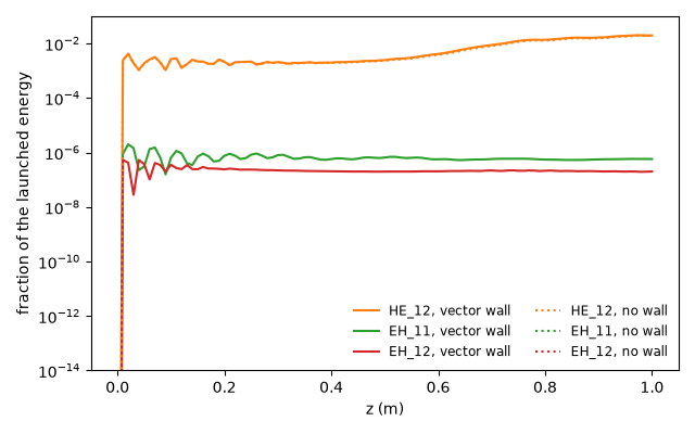
vector wall: HE_11 6.71e-01, HE_12 1.98e-02, EH_11 5.76e-07, EH_12 2.02e-07
no wall    : HE_11 6.58e-01, HE_12 1.95e-02, EH_11 6.96e-35, EH_12 2.58e-33

Runtime and reproducibility

Four complete one-metre runs of three or four coupled modes.

settings = te.metadata.backend.settings
print(
    f"{time.perf_counter() - started:.0f} s; backend {te.metadata.backend.name}, "
    f"{settings.get('thread_count', 'default')} threads"
)

314 s; backend native, 4 threads

Related reading

Continue with Vector boundary response for the model, options and limits, and Assessing numerical accuracy for convergence checks. For a paced propagation lesson, return to Resonant dispersive-wave propagation.