Radial diffraction and a separate self-focusing diagnostic#

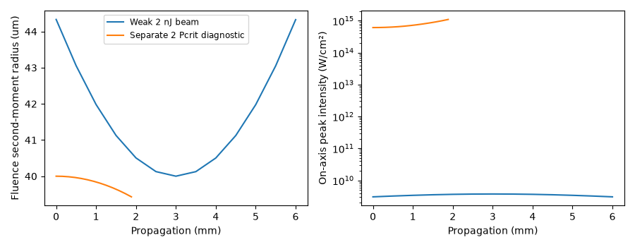
The first beam is a weak one: argon at 1.2 bar, 800 nm, 20 fs, 2 nJ in the argon, and a 40 um waist. This reduced calculation uses 128 radial samples within 0.6 mm and propagates 6 mm from a launch focused as in vacuum, 3 mm before the waist. A 2 nJ pulse is far below the critical power for self-focusing.

The second, separately labelled calculation launches a collimated beam whose peak field on axis, \(6.78\times10^{10}\) V/m, carries twice the Townes critical power. It demonstrates initial contraction, stopping before collapse. Neither its peak intensity nor its stopping plane is a convergence claim. See The free-space model for the power derivation and limitations, and Energy and flux in a medium for how energy and power are measured in the argon.

import matplotlib.pyplot as plt
import numpy as np

from solprop.constants import C
from solprop.driver import Simulation, SimulationSettings
from solprop.grid import EnvelopeGrid, RadialGrid
from solprop.nonlinear.responses import KerrResponse
from solprop.physdata import chi3, gamma3, refractive_index
from solprop.pulses import GaussianPulse, SpatialPulse
from solprop.spatial import (
    SpatialFlux,
    SpatialMedium,
    critical_power,
    spatial_energy,
    spatial_power,
)
from solprop.stats import StatsSpec
from solprop.stepper import PIController

Both calculations use the envelope Kerr response, with no third harmonic, plasma or Raman term. Material-range diagnostics remain visible when the numerical guard band extends beyond the published gas-index fit.

medium = SpatialMedium("Ar", pressure=1.2)
space = RadialGrid(600e-6, 128)
responses = [KerrResponse(gamma3("Ar", wavelength=800e-9), thg=False)]
spec = StatsSpec(names=("energy", "on_axis_intensity", "beam_radius"))
length = 6e-3
grid = EnvelopeGrid.from_limits(length, 800e-9, (400e-9, 2e-6), 200e-15, thg=False)
weak_pulse = SpatialPulse(
    GaussianPulse(wavelength=800e-9, fwhm=20e-15, energy=2e-9),
    waist=40e-6,
    propz=-3e-3,
)
settings = SimulationSettings(
    controller=PIController(rtol=1e-6, atol=1e-13),
    save_planes=np.linspace(0, length, 13)[1:],
    dz_init=1e-4,
    dz_max=5e-4,
    stats=spec,
)
# The weak beam is launched with its vacuum focusing -- its waist and wavefront are
# those of a Gaussian beam in vacuum -- although it propagates in argon. That choice
# is made explicitly here; by default a SpatialPulse is built in the entrance
# material. Built in vacuum, its 2 nJ would be a vacuum energy, so the array is
# rescaled to carry 2 nJ through the entrance plane in the argon.
weak_launch = weak_pulse.build(grid, space, medium=SpatialMedium())
entrance = SpatialFlux.resolve(grid, space, medium)
weak_launch *= np.sqrt(2e-9 / spatial_energy(weak_launch, entrance))
weak = Simulation.from_radial(
    grid, space, medium, responses, weak_launch, settings=settings
).run()

The Townes baseline is the physical power in the argon, at its carrier index. A Gaussian has negative paraxial Hamiltonian above 2/1.86226 times this baseline; twice the baseline is above that sufficient threshold. The diagnostic beam is stated by its physical field, a collimated Gaussian with a unit-peak temporal envelope scaled to FIELD; its peak power is measured from it. Marburger’s empirical distance is shown only as a comparison for a collimated, monochromatic paraxial Gaussian.

FIELD = 6.7785e10  # V/m, the peak of the analytic field on axis
index = float(refractive_index("Ar", 2 * np.pi * C / 800e-9, pressure=1.2))
power = critical_power(800e-9, chi3("Ar", pressure=1.2, wavelength=800e-9), index=index)
rayleigh = np.pi * index * (40e-6) ** 2 / 800e-9
diagnostic_length = 0.3 * rayleigh
diagnostic_grid = EnvelopeGrid.from_limits(
    diagnostic_length, 800e-9, (400e-9, 2e-6), 200e-15, thg=False
)
envelope = GaussianPulse(wavelength=800e-9, fwhm=20e-15, peak_power=1.0).build(
    diagnostic_grid
)
profile = np.exp(-((space.r / 40e-6) ** 2))
diagnostic_pulse = FIELD * space.hankel.forward(profile)[:, None, None] * envelope
peak_power = float(
    np.max(
        spatial_power(
            diagnostic_pulse, SpatialFlux.resolve(diagnostic_grid, space, medium)
        )
    )
)
ratio = peak_power / power
marburger = 0.367 * rayleigh / np.sqrt((np.sqrt(ratio) - 0.852) ** 2 - 0.0219)
diagnostic_settings = SimulationSettings(
    controller=PIController(rtol=1e-6, atol=1e-13),
    save_planes=np.linspace(0, diagnostic_length, 13)[1:],
    dz_init=1e-5,
    dz_max=diagnostic_length / 12,
    stats=spec,
)
diagnostic = Simulation.from_radial(
    diagnostic_grid,
    space,
    medium,
    responses,
    diagnostic_pulse,
    settings=diagnostic_settings,
).run()
print(f"Townes baseline: {power * 1e-9:.6g} GW; diagnostic: {peak_power * 1e-9:.6g} GW")
print(f"P/Pcr = {ratio:.4f}")
print(f"weak beam energy: {np.ravel(weak['stats/energy'])[0] * 1e9:.4f} nJ")
print(f"Marburger comparison (non-gating): {marburger * 1e3:.6g} mm")

Townes baseline: 7.66561 GW; diagnostic: 15.3312 GW
P/Pcr = 2.0000
weak beam energy: 2.0000 nJ
Marburger comparison (non-gating): 4.25276 mm

The width is a second moment of the time-integrated axial flux. The weak beam focuses near its imposed waist plane; the high-power diagnostic starts at its waist and contracts because of the Kerr response.

figure, axes = plt.subplots(1, 2, figsize=(9, 3.5))
for run, label in (
    (weak, "Weak 2 nJ beam"),
    (diagnostic, "Separate 2 Pcrit diagnostic"),
):
    z = np.asarray(run["z"])
    radius = np.asarray(run["stats/beam_radius"])[..., 0].reshape(-1)
    intensity = np.asarray(run["stats/on_axis_intensity"]).reshape(-1)
    axes[0].plot(z * 1e3, radius * 1e6, label=label)
    axes[1].semilogy(z * 1e3, intensity * 1e-4, label=label)
axes[0].set(xlabel="Propagation (mm)", ylabel="Fluence second-moment radius (um)")
axes[1].set(xlabel="Propagation (mm)", ylabel="On-axis peak intensity (W/cm²)")
axes[0].legend(fontsize="small")
figure.tight_layout()

Radial diffraction and a separate self-focusing diagnostic#

Related reading#