Compare a carrier-resolved pulse with envelope plasma#

Both runs use the same instantaneous argon rate, optmat’s recommended model (OptmatRate), 800 nm, 60 fs intensity FWHM, 1 mJ pulse energy and a 125 um capillary radius. The 8 um propagation distance keeps this deterministic illustration short. Kerr, Raman and third harmonics are absent. This compares two propagation models using the same atomic rate; it does not establish the rate’s accuracy for an experiment.

The envelope population averages the rate around each optical cycle. Its plasma currents retain their separate frequency dependence. The field model resolves the real carrier and its ionisation peaks directly. The fundamental spectral comparison uses physical angular frequency and spectral energy density on both grids. No stochastic noise is added.

This is a single-resolution example with an explicit 1% population discrepancy budget for this chosen pulse; how the discrepancy depends on bandwidth, depletion per cycle, sampling and integration step is a separate convergence question. An FFT collar beyond argon’s refractive-index fit raises a MaterialRangeWarning, retained in the gallery output.

from time import perf_counter

import matplotlib.pyplot as plt
import numpy as np

from solprop.boundaries import absorber
from solprop.driver import Simulation, SimulationSettings
from solprop.grid import EnvelopeGrid, FieldGrid
from solprop.modes import MarcatiliMode
from solprop.nonlinear import EnvelopePlasmaResponse
from solprop.nonlinear.optmat_rates import OptmatRate
from solprop.nonlinear.responses import PlasmaResponse
from solprop.processing import get_spectral_density, species_ionisation
from solprop.pulses import GaussianPulse
from solprop.stats import StatsSpec
from solprop.stepper import FixedSchedule, PIController

started = perf_counter()
length = 8e-6
mode = MarcatiliMode(125e-6, "Ar", 1.0, cladding=1.45, loss=False)
pulse = GaussianPulse(wavelength=800e-9, fwhm=60e-15, energy=1e-3)
field_grid = FieldGrid.from_limits(length, 800e-9, (500e-9, 1.2e-6), 320e-15, ffac=16)
envelope_grid = EnvelopeGrid.from_limits(length, 800e-9, (500e-9, 1.2e-6), 320e-15)
rate = OptmatRate("Ar", 800e-9)
runs = {}
for label, grid, response in (
    ("Carrier resolved", field_grid, PlasmaResponse("Ar", rate)),
    ("Envelope", envelope_grid, EnvelopePlasmaResponse("Ar", rate)),
):
    simulation = Simulation(
        grid,
        mode,
        [response],
        pulse,
        settings=SimulationSettings(
            backend="numpy_ref",
            controller=PIController(rtol=1e-6, atol=1e-14),
            save_planes=np.linspace(length / 4, length, 4),
            dz_init=length / 4,
            dz_max=length / 4,
            schedule=FixedSchedule.uniform(0.0, length, length / 4),
            ionisation_field_range=(1e7, 1e11),
            # The pulse fits far inside this collar. Its reference length keeps
            # explicit collar damping stable over the four steps of this short slab.
            absorber=absorber(grid, boundary_length=1e-3),
            stats=StatsSpec(
                names=("energy", "species_ionisation", "peak_ionisation_rate")
            ),
        ),
    )
    runs[label] = simulation.run(progress="none")

Fractions are evaluated at the end of each local pulse at every saved plane.

figure, axes = plt.subplots(1, 2, figsize=(10, 3.5))
for label, output in runs.items():
    axes[0].plot(
        output["z"] * 1e6, species_ionisation(output)[:, 0, 0], "o-", label=label
    )
    wavelength, density = get_spectral_density(output, plane=-1, modes="sum")
    axes[1].plot(wavelength * 1e9, density * 1e-9, label=label)
axes[0].set(xlabel="Distance (um)", ylabel="Final ionised fraction")
axes[1].set(xlabel="Wavelength (nm)", ylabel="Spectral energy (J/nm)", xlim=(740, 860))
axes[0].legend()
axes[1].legend()
figure.tight_layout()

carrier_fraction = species_ionisation(runs["Carrier resolved"])[-1, 0, 0]
envelope_fraction = species_ionisation(runs["Envelope"])[-1, 0, 0]
discrepancy = abs(envelope_fraction - carrier_fraction) / carrier_fraction
assert discrepancy < 0.01
print(f"Final population discrepancy: {discrepancy:.3%}")
print(f"Complete example: {perf_counter() - started:.3f} s")
plt.show()

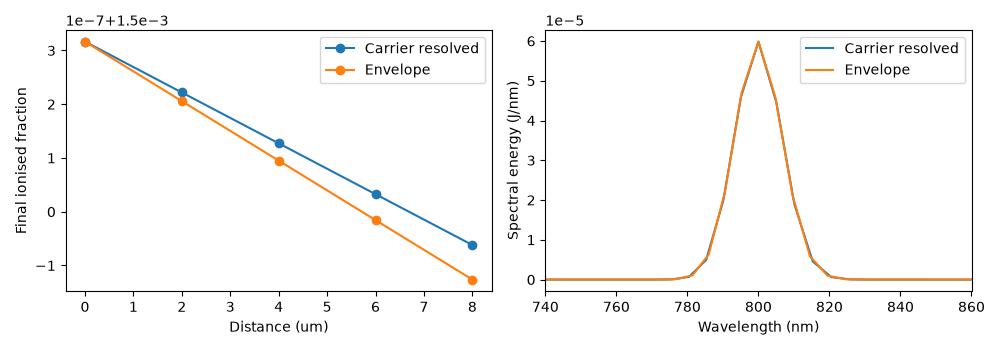
Final population discrepancy: 0.004%
Complete example: 1.586 s

Compare a carrier-resolved pulse with envelope plasma#

Related reading#