Note
Go to the end to download the full example code.
A four-wave-mixing delay scan through one backend#
Two equal pulses cross at a small angle in a thin Kerr sample. Where they overlap in space and time the cubic response writes a transient grating, and each beam diffracts from it into a new direction: the self-diffraction signals of degenerate four-wave mixing. Scanning the delay of one beam and recording the signal’s energy traces their correlation, which is how such measurements characterise pulses.
The scan runs the same translated problem for many inputs, and every saved plane is wanted only as statistics. This tutorial builds it the memory-lean way (Running a simulation, Output: what a run leaves behind):
one backend constructed once, by
runner(), and one input loaded into it per delay;statistics-only planes,
fields="none", with the beams and signals read fromregion_spectrumboxes of transverse wavevector;a custom spectral absorber,
custom_absorber(), for an absorption band of the sample;a transverse safety ramp,
TransverseCollar.
It then shows why the grid, not the ramp, keeps the cubic products from aliasing, and checks the grid by refinement. The sample is a generic dispersionless glass, so the correlation has a closed form to compare with.
Scales and the one-half rule#
The pulses are 50 fs long at 800 nm with a 50 μm waist and a peak field of \(9.49\times10^8\) V/m each, about 0.36 μJ each in the sample (printed below); the sample is 1 mm of a medium of constant index 1.45 with an illustrative nonlinear index of \(3\times10^{-20}\) m²/W. Inside it the beams travel at \(\pm15\) mrad, so their transverse wavenumbers are \(\pm K_0\) with \(K_0 = nk_0\sin\theta\). The signal \(2\mathbf k_1-\mathbf k_2\) leaves at \(3K_0\), and its mirror \(2\mathbf k_2-\mathbf k_1\) at \(-3K_0\).
A periodic grid of spacing \(\Delta x\) holds \(|k_x| \le k_{x,\max} = \pi/\Delta x\). A cubic product of content within \(|k_x|\le K\) reaches \(3K\), and the discrete product is generated already folded back into the grid at \(k-2k_{x,\max}\). The folded products stay out of the energetic band only while \(K<k_{x,\max}/2\), the one-half rule (Cartesian free-space propagation). The energetic content is the two beams and, once generated, the signals: \(K\) is \(3K_0\) plus the signal’s spread, about \(3.5K_0\), so the rule asks for \(k_{x,\max} > 7K_0\), a spacing below 2.6 μm. A spacing of 2 μm puts \(K_0\) at 0.11 of \(k_{x,\max}\) and the signal at 0.33. In y the beams’ own spread decides, and 15 μm suffices.
import time

import matplotlib.pyplot as plt
import numpy as np

from solprop.boundaries import TransverseCollar, absorber, custom_absorber
from solprop.constants import C
from solprop.driver import Simulation, SimulationSettings
from solprop.grid import EnvelopeGrid, FreeGrid
from solprop.nonlinear.responses import KerrResponse
from solprop.physdata.nonlinear_data import chi3_from_n2
from solprop.pulses import GaussianPulse
from solprop.spatial import SpatialFlux, SpatialMedium, spatial_energy
from solprop.stats import StatsSpec
from solprop.stepper import FixedSchedule, PIController

started = time.perf_counter()
LENGTH = 1e-3
WAVELENGTH = 800e-9
INDEX = 1.45
N2 = 3e-20
WAIST = 50e-6
FIELD = 9.4934e8  # V/m, the peak of each beam's analytic field
FWHM = 50e-15
ANGLE = 0.015
K0 = 2 * np.pi * INDEX / WAVELENGTH * np.sin(ANGLE)
grid = EnvelopeGrid.from_limits(LENGTH, WAVELENGTH, (740e-9, 870e-9), 300e-15)


def transverse_grid(spacing, n_y=16):
    """A 0.3 mm by 0.24 mm box at the given x spacing, without a real-space collar."""
    return FreeGrid(0.15e-3, round(0.3e-3 / spacing), 0.12e-3, n_y, window_factor=0.0)


space = transverse_grid(2e-6)
k_max = float(np.max(np.abs(space.k_x)))
print(
    f"K0 = {K0:.3e} rad/m; K0/k_max = {K0 / k_max:.2f}; signal at {3 * K0 / k_max:.2f}"
)
print(f"grid: {space.n_x} x {space.n_y} columns, {grid.n_omega} frequencies")
K0 = 1.708e+05 rad/m; K0/k_max = 0.11; signal at 0.33
grid: 150 x 16 columns, 128 frequencies
Build the launch#
An array launch is the transverse DFT of each frequency’s field, shape
(n_x*n_y, n_pol, n_omega) in the internal FFT convention, whose tilt carries a
minus sign (the Two crossing beams in Cartesian free space lesson derives
it). Beam 1 travels towards positive x; beam 2, towards negative x, is delayed by
t0, positive for later arrival. Each beam is stated by its physical field: a
Gaussian times a temporal envelope of unit peak, scaled to FIELD. Its energy is
then what it carries through the sample’s entrance, the axial Poynting flux in the
glass (Energy and flux in a medium).
def beam(spatial_grid, direction, delay=0.0):
    """One tilted Gaussian beam of peak field FIELD on its grid."""
    x, y = np.meshgrid(spatial_grid.x, spatial_grid.y)
    pulse = GaussianPulse(wavelength=WAVELENGTH, fwhm=FWHM, peak_power=1.0, t0=delay)
    profile = np.exp(-(x**2 + y**2) / WAIST**2)
    tilt = np.exp(
        -1j * direction * x[..., None] * grid.omega * INDEX * np.sin(ANGLE) / C
    )
    physical = FIELD * profile[..., None] * tilt * pulse.build(grid)[0, 0]
    return np.fft.fft2(physical, axes=(0, 1)).reshape(-1, 1, grid.n_omega)


def launch(spatial_grid, delay=0.0):
    """Both beams, beam 2 delayed by `delay` in s."""
    return beam(spatial_grid, +1) + beam(spatial_grid, -1, delay)


glass = SpatialMedium(INDEX)
energy = spatial_energy(beam(space, +1), SpatialFlux.resolve(grid, space, glass))
print(f"each beam carries {energy * 1e6:.4f} μJ into the sample")
each beam carries 0.3625 μJ into the sample
Statistics, absorber and collar#
Four boxes of transverse wavevector collect the two beams and the two signals,
each one \(K_0\) wide in \(k_x\) and open in \(k_y\); with
fields="none" no plane stores or transfers a field, and region_spectrum is
computed from the live state.
The sample absorbs on the short-wavelength side: a power absorption coefficient
rising smoothly to 3000 m⁻¹ below about 770 nm. custom_absorber adds it to a
collar’s spectral rate. A spectral rate is diagonal in frequency, so it is folded
into the linear operator, exact and free whatever the step
(Absorbing boundaries). The collar here is spectral-only
(temporal=False): the medium has no dispersion, so nothing walks to the edge of
the time window, and a collar that absorbs nothing in time compiles no temporal pass.
The beams stay well inside the box too, so the grid has no real-space collar
(window_factor=0).
The transverse collar ramps a power rate up to 20 000 m⁻¹ over the outer tenth of the grid’s wavenumbers, which removes 60 dB of field at the edge over about 0.7 mm. On this grid nothing physical reaches that band; the ramp is a safety net against content creeping towards the Nyquist edge.
The steps are replayed, eight per run, so every delay takes the same schedule.
regions = np.array(
    [
        [0.5 * K0, 1.5 * K0, -np.inf, np.inf],  # beam 1
        [-1.5 * K0, -0.5 * K0, -np.inf, np.inf],  # beam 2
        [2.5 * K0, 3.5 * K0, -np.inf, np.inf],  # signal 2k1 - k2
        [-3.5 * K0, -2.5 * K0, -np.inf, np.inf],  # signal 2k2 - k1
    ]
)
edge = 2 * np.pi * C / 770e-9


def absorption(omega):
    """The sample's power absorption coefficient in 1/m."""
    return 3e3 / (1 + np.exp(-(omega - edge) / 2e13))


band_absorber = custom_absorber(grid, absorption, collar=absorber(grid, temporal=False))


def settings_for(**changes):
    """The scan's settings, with `changes` applied."""
    step = LENGTH / 8
    options = {
        "controller": PIController(rtol=1e-6, atol=1e-12),
        "save_planes": [LENGTH],
        "dz_init": step,
        "dz_max": step,
        "schedule": FixedSchedule.uniform(0.0, LENGTH, step, save_planes=[LENGTH]),
        "stats": StatsSpec(
            names=("energy", "region_spectrum"), spectral_regions=regions
        ),
        "absorber": band_absorber,
        "transverse_absorber": TransverseCollar(2e4),
        "fields": "none",
    }
    options.update(changes)
    return SimulationSettings(**options)


def simulation_for(spatial_grid, **changes):
    """The sample and its responses on `spatial_grid`."""
    return Simulation.from_free(
        grid,
        spatial_grid,
        glass,
        [KerrResponse(chi3_from_n2(N2, INDEX), thg=False)],
        launch(spatial_grid),
        settings=settings_for(**changes),
    )
The scan#
The runner translates, admits the memory and builds the backend once; each delay
is one run on it, with the delay recorded in that run’s configuration and hash.
The energy in each box is the region spectrum summed over frequency.
delays = np.linspace(-75e-15, 75e-15, 11)
energies = []
simulation = simulation_for(space)
with simulation.runner() as runner:
    for delay in delays:
        output = runner.run(
            launch(space, delay), configuration={"delay": delay}, progress="none"
        )
        spectrum = np.asarray(output["stats/region_spectrum"])[-1]
        energies.append(spectrum.sum(axis=-1) * grid.d_omega)
energies = np.array(energies)
efficiency = energies[:, 2] / (energies[:, 0] + energies[:, 1])
print(f"peak signal efficiency: {efficiency.max():.2e} of the beams' energy")
peak signal efficiency: 3.49e-04 of the beams' energy
In the weak-conversion limit the signal \(2\mathbf k_1-\mathbf k_2\) is driven by \(E_1^2E_2^*\), so its energy follows \(\int I_1^2(t)\,I_2(t-\tau)\,dt\). For Gaussian pulses of intensity FWHM \(T\) that is a Gaussian in \(\tau\) of FWHM \(T\sqrt{3/2}\), 61 fs here; the medium has no dispersion to change it. The scan’s second moment, read as a Gaussian’s width, recovers it.
centre = np.sum(delays * efficiency) / np.sum(efficiency)
width = (
    2
    * np.sqrt(2 * np.log(2))
    * np.sqrt(np.sum((delays - centre) ** 2 * efficiency) / np.sum(efficiency))
)
predicted = FWHM * np.sqrt(1.5)
print(f"correlation FWHM: {width * 1e15:.1f} fs (predicted {predicted * 1e15:.1f} fs)")
fine = np.linspace(delays[0], delays[-1], 200)
figure, axis = plt.subplots(figsize=(6, 3.6), layout="constrained")
axis.plot(delays * 1e15, efficiency, "o", label="scan")
axis.plot(
    fine * 1e15,
    efficiency.max() * np.exp(-4 * np.log(2) * (fine - centre) ** 2 / predicted**2),
    label=r"$\int I_1^2 I_2$, Gaussian pulses",
)
axis.set(xlabel="delay of beam 2 (fs)", ylabel="signal / beam energy")
axis.legend()
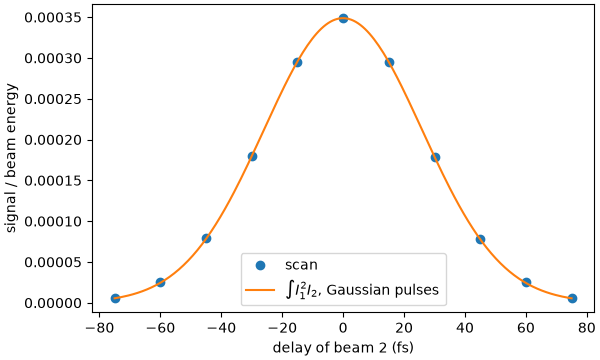
correlation FWHM: 61.1 fs (predicted 61.2 fs)

<matplotlib.legend.Legend object at 0x71a0b168f0e0>
Grid sizing, not the collar, prevents aliasing#
On a grid of 7.4 μm the beams sit at \(0.40\,k_{x,\max}\), at the edge of the
one-half rule once their spread is counted, and the signal at
\(1.2\,k_{x,\max}\), past the grid’s edge. It is generated already folded, at
\(3K_0-2k_{x,\max} \approx -0.8\,k_{x,\max} \approx -2K_0\): an unphysical beam
on the wrong side, at an angle where a cubic product of the two beams, landing only
on odd multiples of \(K_0\), puts nothing. It lands where the collar’s ramp is
exactly zero, because the fold happens inside the product’s evaluation, so the collar
cannot touch it. Each run below keeps its exit field (fields="planes",
field_planes=(-1,)) to show the transverse spectrum.
def kx_spectrum(spatial_grid, run):
    """The exit plane's energy per k_x column, summed over k_y and frequency."""
    field = run.plane_field(-1, convention="fft")
    # Each column and bin weighted by its real axial admittance in the glass.
    flux = SpatialFlux.resolve(grid, spatial_grid, glass, z=LENGTH)
    weighted = np.real(flux.admittance()) * np.sum(np.abs(field) ** 2, axis=1)
    density = np.sum(weighted, axis=1).reshape(spatial_grid.n_y, spatial_grid.n_x)
    profile = density.sum(axis=0)
    return np.fft.fftshift(spatial_grid.k_x), np.fft.fftshift(profile / profile.sum())


coarse = transverse_grid(7.4e-6)
cases = {
    "7.4 μm, no collar": (coarse, None),
    "7.4 μm, collar": (coarse, TransverseCollar(2e4)),
    "2 μm, collar": (space, TransverseCollar(2e4)),
}
figure, axis = plt.subplots(figsize=(7, 3.8), layout="constrained")
for label, (spatial_grid, collar) in cases.items():
    run = simulation_for(
        spatial_grid,
        fields="planes",
        field_planes=(-1,),
        transverse_absorber=collar,
    ).run(progress="none")
    k_x, profile = kx_spectrum(spatial_grid, run)
    axis.semilogy(k_x / K0, profile, ".-", ms=3, label=label)
    folded = np.sum(profile[np.abs(np.abs(k_x) / K0 - 2) < 0.25])
    print(f"{label}: energy fraction within K0/4 of +-2 K0: {folded:.2e}")
axis.set(xlabel=r"$k_x / K_0$", ylabel="energy fraction per column", ylim=(1e-12, 1))
axis.axvline(3, color="0.6", lw=0.8)
axis.axvline(-3, color="0.6", lw=0.8)
axis.legend()
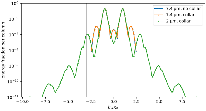
7.4 μm, no collar: energy fraction within K0/4 of +-2 K0: 5.44e-03
7.4 μm, collar: energy fraction within K0/4 of +-2 K0: 5.29e-03
2 μm, collar: energy fraction within K0/4 of +-2 K0: 1.29e-05

<matplotlib.legend.Legend object at 0x71a0b168fe00>
On the coarse grid the alias carries the same energy with and without the collar, to within the little the ramp takes from the beams’ and the alias’s own far tails: it has nothing else to act on. On the 2 μm grid the band at \(\pm2K_0\) holds only the far tails of the beams, broadened by self- and cross-phase modulation, and the signal stands at \(\pm3K_0\) (grey lines), where it belongs.
Refinement checks the grid#
Refinement judges the grid: the same box at a finer spacing must leave the result where it was. The signal efficiency at zero delay on a 3 μm grid, which breaks the one-half rule for the signal (\(k_{x,\max} = 6.1K_0 < 7K_0\)), on the scan’s grid, and on a grid finer in both directions:
refined = {
    "3 μm x 15 μm": transverse_grid(3e-6),
    "2 μm x 15 μm": space,
    "1.5 μm x 10 μm": transverse_grid(1.5e-6, n_y=24),
}
results = {}
for label, spatial_grid in refined.items():
    run = simulation_for(spatial_grid).run(progress="none")
    spectrum = np.asarray(run["stats/region_spectrum"])[-1].sum(axis=-1)
    results[label] = spectrum[2] / (spectrum[0] + spectrum[1])
reference = results["1.5 μm x 10 μm"]
for label, value in results.items():
    print(f"{label}: {value:.6e}, {value / reference - 1:+.1e} from the finest")
3 μm x 15 μm: 3.492855e-04, +1.7e-03 from the finest
2 μm x 15 μm: 3.487194e-04, +9.2e-05 from the finest
1.5 μm x 10 μm: 3.486872e-04, +0.0e+00 from the finest
The 3 μm grid is off by about a part in a thousand: there the signal’s own cubic products fold onto the other signal. The scan’s grid is within about a part in ten thousand of the finest, far below what the correlation width needs.
The absorption band#
The absorber’s rate is exact in the linear operator, so a beam’s transmitted spectrum falls by \(e^{-\alpha(\omega)L}\) from the launch, with \(\alpha\) the absorber’s whole spectral rate (the band and the collar’s edges). At the scan’s energy self-phase modulation reshapes the spectrum as well; a copy of beam 1 a hundred times weaker in field, one more input to a runner, is linear to about a part in a million and shows the rate alone.
with simulation.runner() as runner:
    alone = runner.run(1e-2 * beam(space, +1), progress="none")
transmitted = np.asarray(alone["stats/region_spectrum"])[:, 0]
order = np.argsort(grid.omega)
omega = grid.omega[order]
ratio = transmitted[-1][order] / np.maximum(transmitted[0][order], 1e-300)
expected = np.exp(-band_absorber.spectral_rate[order] * LENGTH)
bright = transmitted[0][order] > 1e-6 * transmitted[0].max()
print(
    f"largest departure of the transmission from exp(-alpha L): "
    f"{np.max(np.abs(ratio[bright] / expected[bright] - 1)):.1e}"
)
figure, axis = plt.subplots(figsize=(6, 3.6), layout="constrained")
wavelength = 2 * np.pi * C / omega[bright] * 1e9
axis.plot(wavelength, ratio[bright], label="beam 1, exit / entrance")
axis.plot(wavelength, expected[bright], "--", label=r"$e^{-\alpha L}$")
axis.set(xlabel="wavelength (nm)", ylabel="transmission")
axis.legend()
print(f"tutorial run time: {time.perf_counter() - started:.1f} s")
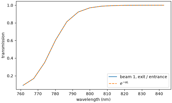
largest departure of the transmission from exp(-alpha L): 1.3e-06
tutorial run time: 24.1 s