Package overview#

Check the installation, see which backend a run will use, and propagate a pulse: a two-centimetre run through a helium-filled capillary, read back through the same accessors every later example uses. The tutorials that follow take each part in turn – pulses, analysing a run, the interactive namespace and scans; then gas-filled capillaries, other waveguides, free space and the compression tools – and the guide says which model to use for what.

The package version, and the backend backend="auto" resolves to here: native where the solprop-native package is installed, otherwise numba_cpu.

import warnings

import matplotlib.pyplot as plt
import numpy as np

import solprop
from solprop.backends.registry import available, resolve_name
from solprop.driver import prop_capillary
from solprop.exceptions import MaterialRangeWarning
from solprop.processing import energy, fwhm_t, get_spectral_density

print(f"solprop {solprop.__version__}")
print(f"installed backends {available()}; auto resolves to {resolve_name('auto')}")

solprop 0.0.1.dev244+g938cb81bb
installed backends ('numpy_ref', 'numba_cpu'); auto resolves to numba_cpu

One call builds the grid, the mode, the gas, the responses and the pulse, and runs them: two centimetres of a 125 um helium-filled capillary at 1 bar, pumped by a 10 fs, 20 uJ pulse at 800 nm. The gas index is asked for beyond its fitted range at the short end of the window, which it reports; that notice is silenced.

with warnings.catch_warnings():
    warnings.simplefilter("ignore", MaterialRangeWarning)
    run = prop_capillary(
        125e-6,
        0.02,
        "He",
        1.0,
        lambda0=800e-9,
        wavelength_limits=(200e-9, 2e-6),
        trange=150e-15,
        fwhm=10e-15,
        energy=20e-6,
        n_save=5,
        progress="none",
    )
print(run)

MemoryOutput
  state:           closed
  planes:          5, 0 m to 20 mm
  field per plane: 1 x 1 x 513 (modes x components x omega)
  statistics:      core_radius, density, electron_density, energy, fwhm_t, fwhm_t_out...
  between planes:  none
  run:             RunMetadata(multimode, field grid of 1024, 1 modes, numba_cpu, 202...

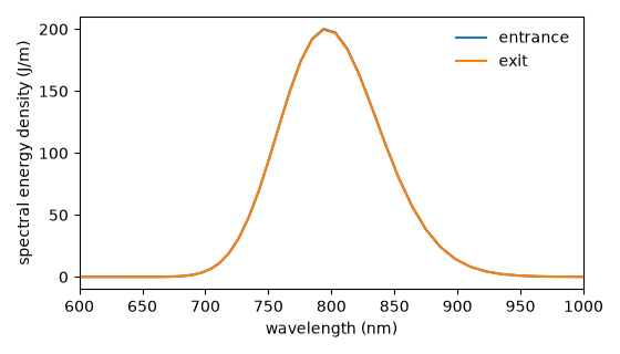
The run is read through solprop.processing: the energy and duration at each save plane, and the spectrum at the entrance and the exit. At this energy and length the pulse barely changes, which is the point: every later example reads a run the same way.

print("energy (uJ):", np.round(np.asarray(energy(run)).ravel() * 1e6, 4))
print("duration (fs):", np.round(np.asarray(fwhm_t(run)).ravel() * 1e15, 3))

fig, ax = plt.subplots(figsize=(5.6, 3.2))
for plane, label in ((0, "entrance"), (-1, "exit")):
    wavelength, density = get_spectral_density(run, "wavelength", plane=plane)
    order = np.argsort(wavelength)
    ax.plot(wavelength[order] * 1e9, np.ravel(density)[order], label=label)
ax.set_xlim(600.0, 1000.0)
ax.set_xlabel("wavelength (nm)")
ax.set_ylabel("spectral energy density (J/m)")
ax.legend(frameon=False)
fig.tight_layout()

energy (uJ): [20.     19.9857 19.9715 19.9572 19.943 ]
duration (fs): [10.001  9.995  9.978  9.965  9.946]

Package overview#

Related reading#