Assessing numerical accuracy

A solver tolerance controls part of a calculation’s numerical error. It does not choose an adequate time window, resolve a narrow spatial feature, validate a material model or compensate for omitted modes. Assess accuracy against the quantity you intend to use: a band energy, pulse duration, conversion efficiency, complex field or spatial intensity can converge at different rates.

The soliton lesson uses recurrence and energy conservation as checks. The crossing-beam lesson compares superposition, beam motion, fringe spacing and spatial refinement. These checks are useful because each has a reference independent of the plotted appearance.

Change one resolution at a time

Keep the physical problem and the measurement fixed while changing its numerical representation. Compare results at the same propagation positions and with the same spectral windows and field conventions.

Control	What it resolves	Useful comparison
rtol, atol, and a step cap	Evolution along the propagation direction	Tighten tolerances or reduce dz_max; compare the chosen observable
Temporal sample spacing and response oversampling	Carrier, pulse structure and nonlinear products	Refine the sampled response while retaining the same physical window
Time-window duration	Walk-off, delayed response and pulse tails	Enlarge the window, preserving adequate sample spacing and an unaffected measurement region
Frequency band and spectral collar	Generated frequencies and their absorption	Extend the band; inspect energy and signal near the collar
Number of modes	Accessible guided fields and intermodal transfer	Add physically relevant modes while resolving their overlap integrals
Transverse quadrature	Local nonlinear response within the retained modes	Increase nodes independently of mode count
Spatial spacing and extent	Diffraction, fringes, focusing and boundaries	Refine spacing and enlarge the domain as separate checks
Operator tables and longitudinal sections	Varying dispersion, geometry and coupling	Tighten table tolerance or refine sections, alongside propagation-step refinement

An embedded radial indicator compares two related quadrature rules. Both can miss the same feature, so a small indicator is useful evidence but does not replace an independent refinement. See transverse quadrature and expensive-response radial rules.

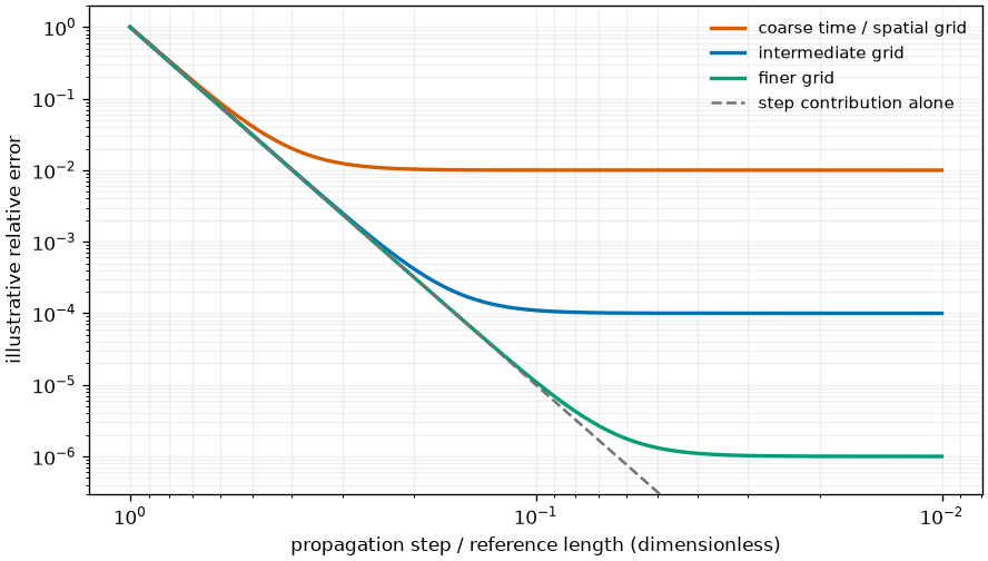
Illustrative error budget, not a measured convergence order. Each curve is the sum of a fifth-power step contribution and a fixed grid contribution. Reducing the propagation step cannot remove a temporal or spatial discretisation error. The actual order and floor must be measured for the problem and observable.

Interpret differences and conservation checks

Use at least three resolution levels when estimating a convergence order. Two levels show a difference, but cannot by themselves establish the asymptotic rate or exclude a shared bias. An observed plateau can come from another unresolved axis, material interpolation, floating-point error or the observable’s definition.

Energy conservation is valuable for a lossless model, but a conserving method can still have phase or pulse-shape errors. With ionisation, Raman energy exchange, waveguide loss or absorbing boundaries, optical energy need not be conserved. Check the expected energy accounting and the loss channels instead of treating every decrease as a solver defect. The power and intensity definitions specify the measured energy.

For a weak generated band, report both its absolute energy and a relative difference. A large percentage difference in an almost empty band and a small percentage error in the total field can describe the same result. For complex fields, state whether comparisons permit a global phase or time shift; aligning curves removes those errors from the measurement.

Tolerances, boundaries and coupled propagation

The solver error norm scales a local estimate. Its tolerance is not a guaranteed global error bound, and equal tolerances in two methods do not promise equal accuracy. Compare measured errors when choosing between Adams and Runge–Kutta.

Keep significant light away from an absorbing collar unless the observable deliberately measures the remaining field after that absorption. A smooth absorber reduces wraparound; it also changes any light reaching it. Increasing absorber strength cannot recover discarded physics.

For a coupled linear problem with no nonlinear source, the current exponential Adams path has a limitation: its frozen-block residual is not controlled by the ordinary source error estimate. Refine dz_max or use the Runge–Kutta route as described under Adams limitations. Tapers also require convergence of the local modes and their longitudinal interpolation.

Finally, distinguish numerical agreement from physical validity. Two backends can agree on the same approximation; a refined calculation can still use extrapolated material data or omit a relevant degree of freedom. The material validity chapters and the selected geometry’s limitations complete the assessment.