Offline optics and compression

A propagation ends with a pulse that still has to get to an experiment: through a window, down a beam line in air, off a set of chirped mirrors, through a pair of wedges. solprop.optics describes those linear elements and solprop.processing.compression searches their parameters for the shortest pulse. Together they cover a Taylor-expanded spectral phase, a thickness of glass or gas, chirped mirrors, grating pairs and prism pairs (the last two with explicit physical tuning coordinates), the compressors that search each of them, and the optimisation of the carrier-envelope phase. Everything here is applied to a saved plane after the run, so no propagation is repeated; read this page to see a simulated pulse as it would arrive at an experiment, or to design the compressor that gets it there. To send the compressed pulse on into another simulation – through focusing optics into a second capillary, say – apply the same elements to a field plane with SpectralTransfer (coupling simulations).

One concept: a transfer function

Every element is a callable \(H(\omega)\) giving the complex amplitude response in the optics convention of the conventions page §2:

\[ \tilde E_{\rm out}(\omega) = H(\omega)\,\tilde E_{\rm in}(\omega),\qquad H = |H|\,e^{+i\varphi(\omega)} . \]

The group delay is \(+d\varphi/d\omega\), positive group-delay dispersion \(d^2\varphi/d\omega^2\) makes the blue arrive later, and a slab of normally dispersive glass chirps positively: textbook signs. The processing layer applies an element to the spectrum in the internal FFT convention (the arrays output.fields("fft") returns), so there it multiplies by \(e^{-i\varphi}\); that crossing is made in exactly one function, stored_factor(), by solprop.fourier.to_internal(). A transfer function is diagonal in frequency, so it commutes with the half-window origin shift between the two conventions and the conjugation is all the crossing needs. The Taylor sum itself is written once, taylor_phase(), and the pulse builders use the same one, so a chirp put on a pulse with phases= is removed exactly by the opposite TaylorPhase.

Tests hold each element to the sign convention: positive GDD broadens a Gaussian to \(\tau\sqrt{1+(4\ln2\,\varphi_2/\tau^2)^2}\) and delays its blue half; a positive delay coefficient arrives later; fused silica has \(+36.16\) fs²/mm at 800 nm and a negative GDD at 1550 nm.

The elements

TaylorPhase is \(\varphi(\omega)=\sum_n c_n(\omega-\omega_0)^n/n!\) with the coefficients zero-based — (CEP, delay, GDD, TOD, ...) in rad, s, s², s³ — the same indexing as the phases= keyword of the pulse builders.

Material is a thickness of glass or a path through a gas,

\[ H = \exp\{+i[\beta(\omega)-\beta_1(\omega_0)(\omega-\omega_0)]L\},\qquad \beta = \omega\,\mathrm{Re}\,n/c . \]

The medium is a GlassIndex, the name of a glass, a built-in gas with its pressure in bar, or a Mixture. The group delay at the reference wavelength is removed so the pulse stays in its window, using the model’s own analytic \(dn/d\omega\) rather than a difference of the index. The constant \(\beta_0\) is kept, so the carrier-envelope phase moves with thickness, as it does in a physical optical path. A negative thickness removes material. By default the element is phase-only; loss=True applies \(\exp(-\omega\,\mathrm{Im}\,n\,L/c)\) as well, which matters wherever the selected material model has appreciable absorption.

ChirpedMirror is a dispersive mirror known by its data sheet. One reflection is \(\sqrt{R(\omega)}\,e^{i\varphi(\omega)}\,W(\omega)\); the phase is built from the measured group-delay dispersion,

\[ \varphi(\omega) = \iint \mathrm{GDD}\,d\omega\,d\omega - (a_0 + a_1(\omega-\omega_0)), \]

by the cumulative trapezoid rule on the data’s own samples (the shipped sets are sampled every 0.04 to 0.3 nm, the Thorlabs group-delay table every 2.7 nm; the rule’s error, \(h^2/12\) times the change of the integrand’s slope across the band, is far below the data’s own noise in every case), less the constant and linear part of a polynomial fitted about the reference wavelength: the two integration constants are an arbitrary phase and an overall delay. A data sheet that gives group delay is integrated once. \(W\) is a Planck taper to zero outside the band the data are trusted on: light outside a mirror’s band is not reflected with a known phase, so it is not reflected; where the band reaches beyond the first or last dispersion sample the phase is unknown and the response is zero too, rather than an extrapolation of the data (the taper leaves almost nothing there either way). mirror.bounces(n) gives \(n\) reflections; a negative \(n\) is the phase-only inverse, for taking a known mirror pair out of a measured pulse, and it too is zero outside the band. mirror.gdd(omega) and mirror.group_delay(omega) read the stored phase back.

Chain multiplies elements, so a window, a path in air and a set of mirrors can be applied as one.

import matplotlib.pyplot as plt
import numpy as np

from solprop.optics import ChirpedMirror

fig, ax = plt.subplots(figsize=(6.0, 3.2))
for name in ("PC70", "HD120"):
    mirror = ChirpedMirror.lookup(name)
    wavelength = np.linspace(mirror.band[1] * 1.03, mirror.band[2] * 0.97, 400)
    omega = 2 * np.pi * 299792458.0 / wavelength
    ax.plot(wavelength * 1e9, mirror.gdd(omega) * 1e30, lw=0.9, label=name)
ax.set_ylim(-400, 200)
ax.set_xlabel("wavelength (nm)")
ax.set_ylabel("GDD per reflection (fs$^2$)")
ax.legend(frameon=False)
fig.tight_layout()

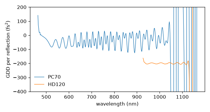
The group-delay dispersion per reflection read back from the stored phase of two of the shipped data sets, inside their bands.

The shipped mirror data

chirped_mirrors() lists seven data sets, which ChirpedMirror.lookup reads and reduces, each with its own reference wavelength, fit order and window, and band.

name	band (nm)	what the file holds
PC70	450–1200	reflectivity and GDD at 5° and 19°; the geometric-mean reflectivity and the mean GDD are used
HD59	1000–1060	GDD only; unit reflectivity
PC147	650–1350	the average per mirror of a complementary pair
PC1611	855–1195	reflectivity and GDD at 7°
PC1821	805–1345	a p-polarised reflectivity beside an s-polarised GDD, by the file’s own column names
HD120	900–1200	reflectivity and GDD, p-polarised at 5°
ThorlabsUMC	650–1050	s-polarised reflectivity and group delay (in fs; integrated once)

The provenance of these data is not recorded: no vendor, part number, data sheet or citation is known for any of them. The files are shipped unchanged, each behind a header that says so. Treat them as what a colleague handed you, and prefer ChirpedMirror.from_data with your own data sheet.

The window glasses

calcium_fluoride(), magnesium_fluoride(), bk7(), sapphire() and barium_fluoride() join fused_silica(), and glass() finds any of them by name; so do the elements and the compressors that name a glass. Each is optmat’s recommended absolute index (SEP 3), and magnesium fluoride and sapphire name their ray (glass("MgF2", axis="o")); a gas path is the gas’s optmat fill. They are described on the materials page.

Looking at a pulse through an element

The time-domain accessors and plots take the element directly, and apply the selections in a fixed order — band pass, then transform limit, then the element:

from solprop.optics import Material
from solprop.plotting import time_1d
from solprop.processing import get_power

window = Material("CaF2", 1e-3, 800e-9)
t, power = get_power(run, plane=-1, transfer=window)
time_1d(run, transfer=window)
time_1d(run, transform_limit=True)

get_field(), get_power(), time_1d() and spectrogram() take transfer=; the first three also transform_limit=. The transform limit is the spectrum’s modulus with zero phase about \(t=0\), the window centre. apply_transfer() returns the spectrum after an element, and transform_limit() the limit’s duration and peak power.

The response is evaluated on the grid’s active band only, and is one elsewhere. A grid usually reaches beyond the range a glass fit is valid over, and the index request then raises a MaterialRangeWarning as it does anywhere else in the package: whether it matters depends on whether your pulse has energy there.

The compressors

Each searches one kind of element for the pulse of highest peak power and returns a Compression: what it found, the element ready for transfer=, and the duration and peak power before, after and at the transform limit. The objective is

\[ J = \frac{\max_t P_{\rm limit}(t)}{\max_t P(t)} \ge 1, \]

with \(P\) the power summed over the selected modes and both polarisation components. \(J=1\) is the transform limit.

compress_taylor() searches orders two to order together, with the carrier-envelope phase and the delay held at zero. The search box is set by the pulse’s own widths: with \(\varphi_2^0=\tau_{\rm lim}\sqrt{|\tau^2-\tau_{\rm lim}^2|}\), the chirp a Gaussian of the measured and limiting widths would carry, order \(n\) is searched within \(\pm\)bound_factor\(\,(\varphi_2^0)^{n/2}\). The widths are the larger of the one read from the half maximum and the one read from the RMS duration, because a pulse with a pedestal has a narrow spike and a long chirp. Order two is a one-parameter search; above it SciPy’s differential evolution runs from the Gaussian estimate, with a fixed seed, and is polished. The same seed gives the same answer.

compress_material() searches a thickness range, which may be negative. The range is scanned on 65 points and the best bracket refined: the objective of a structured pulse has several minima, and a bounded Brent search started blind finds the nearest.

compress_mirrors() tries every number of reflections up to max_reflections, and with a medium optimises its thickness for each count: the mirrors-and-wedges compressor as it stands on a table, where the mirrors over-compensate in whole bounces and glass trims the rest. Its quality includes the mirror’s reflectivity and whatever of the spectrum falls outside its band.

optimise_cep() finds the carrier-envelope phase that maximises the peak of the real field. The phase is periodic, so the circle is scanned and the best sample refined in its own neighbourhood. It is meaningful for a few-cycle pulse only: the peak field of a 30 fs pulse depends on its phase by less than the sampling’s own ripple.

A search that ends on a bound, uses every reflection allowed, or fails is reported in the result (success, message), printed as NOT CLEAN, and logged at WARNING. It never raises for that, and never claims success.

import matplotlib.pyplot as plt

from solprop.processing import compress_taylor, get_power
from solprop.processing._examples import example_output

run = example_output()
found = compress_taylor(run)
fig, ax = plt.subplots(figsize=(6.0, 3.2))
for label, keywords, style in (
    ("as saved", {}, "-"),
    (f"GDD {found.coefficients[2] * 1e30:.0f} fs$^2$", {"transfer": found.transfer}, "-"),
    ("transform limit", {"transform_limit": True}, "k--"),
):
    t, power = get_power(run, plane=-1, oversampling=4, **keywords)
    ax.plot(t * 1e15, power * 1e-6, style, lw=1.2, label=label)
ax.set_xlim(-150, 150)
ax.set_xlabel("time (fs)")
ax.set_ylabel("power (MW)")
ax.legend(frameon=False)
fig.tight_layout()

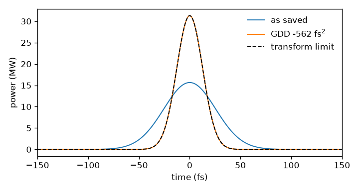
A Gaussian pulse stretched to twice its duration by pure dispersion, as saved, after the Taylor phase found by compress_taylor, and at its transform limit (dashed, under the compressed pulse).

>>> print(found)
Compression by taylor
  found:      GDD -562.2 fs^2
  duration:   60 fs before, 30 fs after, 30 fs at the transform limit
  peak power: 15.66 MW before, 31.31 MW after, 31.31 MW at the limit
  quality:    1 of the transform-limited peak power
  search:     converged: Solution found. (72 evaluations)

The evaluation count is SciPy’s and moves with its version; the tests mask it.

The compressors take an Output (the last plane by default; plane=, modes=, bandpass= select) or, for a pulse that has not been propagated, grid= with the internal-convention spectrum= that pulse.build(grid) returns. compress_taylor searches up to order=2 (the GDD alone) unless told otherwise, compress_material and compress_mirrors need the medium and thickness_range or mirror and max_reflections they search, and optimise_cep takes one mode.

Grating pairs

GratingPair describes two parallel reflection gratings in index-one air. line_density is lines per metre (1200e3 means 1200 lines/mm). separation is the normal surface spacing \(D\), not the slanted inter-grating ray length. Angles are signed radians, with

\[ q(\omega)=\sin\theta_i+\frac{2\pi c m}{d\omega},\qquad \cos\theta_m=\sqrt{1-q^2}>0,\qquad d=1/\rho. \]

The default order is \(m=-1\). littrow_angle() returns \(\arcsin(-m\lambda_0\rho/2)\). double_pass=True means two traversals of the pair, four diffractions; false means one traversal. Write that multiplier as \(N=2\) or \(1\). Treacy’s geometrical path plus the groove phase, referred to a common output plane, gives the following phase up to an affine term:

\[ \phi(\omega)=\frac{ND\omega}{c}\cos\theta_m. \]

The groove phase matters: multiplying the slanted ray length by \(\omega/c\) gives the wrong dispersion. The derivatives are

\[ \phi''=-\frac{NDm^2\lambda^3}{2\pi c^2d^2\cos^3\theta_m},\qquad \frac{\phi'''}{\phi''}=-\frac{3\lambda}{2\pi c} \frac{1-m(\lambda/d)\sin\theta_i-\sin^2\theta_i}{\cos^2\theta_m}. \]

The TOD ratio follows Treacy and Keller’s p. 103 discussion, and solprop’s tests check it by independent differentiation; the coefficient printed in Keller’s Eq. (3.42) differs from it by a factor of two, a discrepancy in the source that is not resolved.

from solprop.optics import GratingPair, littrow_angle
from solprop.processing import compress_gratings

pair = GratingPair(
    line_density=1200e3,
    separation=0.05,  # m, measured normal to the gratings
    incidence_angle=littrow_angle(1200e3, 800e-9),
    wavelength=800e-9,
    band=(650e-9, 1000e-9),
)
# run is an orthogonal modal output; the motor limits are explicit.
found = compress_gratings(run, pair=pair, separation_range=(0.01, 0.10))
print(found.transfer.separation)

D=0 is a zero-phase limit, but still requires a valid diffraction order. A missing or grazing order inside the working band raises OpticsGeometryError.

Prism pairs and laboratory stage coordinates

PrismPair describes identical isosceles glass wedges in index-one air, the second inverted relative to the first. The first prism, its incident beam and its entry point stay fixed. All lengths are metres, all angles radians. medium is a glass name (glass_names()) or a GlassIndex; only its real index is used, which must exceed one. The geometry is a frozen PrismGeometry:

Coordinate	Laboratory meaning
separation \(R\)	Second-prism stage along the reference inter-prism ray, measured from the formal zero-insertion configuration
insertion \(H\)	Translation of the second prism perpendicular to its horizontal base; positive moves it down
first_face_distance \(a\)	Fixed input intersection, measured along the first entry face from its apex
apex_angle \(\alpha\)	The same fixed apex angle for both prisms
incidence_angle \(\theta_i\)	Fixed external incidence on the first entry face

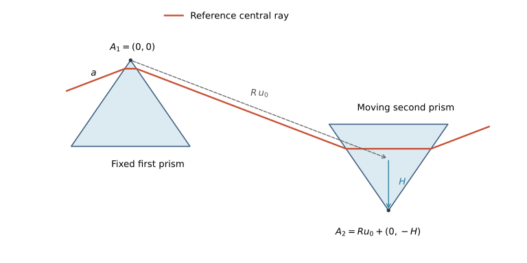
The drawing shows the reference central ray and the two translation directions, with a shortened separation for visibility. Set the first apex to \(A_1=(0,0)\). With \(r=\arcsin(\sin\theta_i/n)\) and \(e=\arcsin[n\sin(\alpha-r)]\), define

\[ u(\omega)=\left(\cos(\alpha/2-e),\ \sin(\alpha/2-e)\right),\qquad A_2=R u(\omega_0)+(0,-H). \]

Thus moving insertion at fixed \(R\) is exactly \(\Delta A_2=(0,-\Delta H)\). pair.apex_distance returns \(|A_2|\); it changes during an insertion scan. Holding \(R\) fixed therefore means holding the separation stage fixed, not holding the actual tip distance or air-ray length fixed.

The exact wavefront phase, up to an affine term, is

\[\phi(\omega)=\frac{N\omega}{c}\,u(\omega)\cdot A_2.\]

Refraction already includes glass dispersion: do not add an extra slab phase. The first-face distance \(a\) changes how much of the total glass lies in each prism, and can make a ray impossible, but it does not change this residual dispersion at fixed apex positions. For arbitrary fixed angles use the full expression above.

For Brewster entry and minimum deviation at the reference, \(\theta_i=\arctan n_0\) and \(\alpha=\pi-2\theta_i\); the helpers brewster_angle() and brewster_apex() return those angles. They remain fixed as frequency and stage settings vary. With \(\delta=e(\omega)-e(\omega_0)\) the same phase becomes

\[ \phi=\frac{N\omega}{c} \left[(R+H\cos\alpha)\cos\delta+H\sin\alpha\sin\delta\right]. \]

This is how Keller’s projected distances relate to these physical stages: the longitudinal and transverse components of \(A_2\) in the reference-ray frame are \(R+H\cos\alpha\) and \(H\sin\alpha\), respectively. The tip distance is their Euclidean norm. These are not interchangeable definitions of separation or insertion.

Calibrating a setup

At the Brewster reference, measure input-face distances \(a\) and \(b\) along each entry face from its apex, and the actual inter-prism air-ray gap \(L\). Then

\[H=\frac{a+b}{2\cos(\alpha/2)},\qquad R=L+H.\]

For other fixed angles, let \(B_1\) be the first exit point and \(g_1=(-\sin(\alpha/2),\cos(\alpha/2))\) the second entry-face direction away from its apex. Recover \(A_2=B_1+Lu_0-bg_1\), then \(R=A_{2x}/u_{0x}\) and \(H=Ru_{0y}-A_{2y}\). Here \(B_1\) can be obtained from the reported first exit-face distance times \((\sin(\alpha/2),-\cos(\alpha/2))\).

pair.ray_paths(omega) returns PrismPaths: both glass lengths for one traversal (also when double_pass=True), the actual air gap, and the first exit, second entry and second exit distances along their faces. The trace requires positive paths and positive face distances, forward refraction at every face and no grazing or total internal reflection. It rejects distances below their floating-point classification uncertainty (\(64\epsilon\) times local coordinate scale divided by intersection sine); it never turns a negative distance into a valid ray. In particular, \(H=0\) with \(a>0\) is a formal mathematical limit, not a feasible ray geometry.

These are central rays through ideal wedges without finite bases. A valid result does not certify a finite beam’s clearance, aperture, absorption, Fresnel transmission or grating efficiency. A one-pass pair retains spatial chirp. Doubling the phase assumes a compensating return or four-prism arrangement; it does not specify a return mirror.

Tuning insertion, then both stages

from solprop.optics import PrismGeometry, PrismPair, brewster_angle, brewster_apex
from solprop.physdata import fused_silica
from solprop.processing import compress_prisms

glass = fused_silica(model="malitson_1965/sellmeier")
pair = PrismPair(
    glass,
    PrismGeometry(
        separation=0.6,
        insertion=0.015,
        first_face_distance=0.003,
        apex_angle=brewster_apex(glass, 800e-9),
        incidence_angle=brewster_angle(glass, 800e-9),
    ),
    wavelength=800e-9,
    band=(650e-9, 1050e-9),
)
insertion_only = compress_prisms(run, pair=pair, insertion_range=(0.01, 0.02))
# R, first-face distance and both angles stay exactly fixed.
print(insertion_only.transfer.geometry)

joint = compress_prisms(
    run, pair=pair, insertion_range=(0.01, 0.02), separation_range=(0.4, 0.8)
)
print(joint.transfer.geometry, joint.transfer.apex_distance)

Omit insertion_range to search separation alone. At least one finite, ordered, nonnegative range is required. Increasing insertion does not universally add positive GDD: the net change depends on the wavelength, material and geometry.

The independent dispersion check uses Arissian–Diels (2007), Eq. (7). For a single traversal, with actual total glass-ray length \(G\) and air-ray length \(L\),

\[ \phi''=\frac{G}{c}(2n'+\omega n'')- \frac{\omega L}{c}(e')^2-\frac{n\omega G}{c}(r')^2. \]

The last, glass angular term is retained. Equation (10) applies at the Brewster reference only. TOD differentiates the whole expression, including the derivatives of \(G\), \(L\), \(r'\) and \(e'\). solprop’s tests reproduce that derivative and the common-output-plane ray trace independently. The printed Eq. (11) appears to misapply the product rule, and the TOD values of the paper’s Table I could not be reproduced, so Table I is not used as a test reference.

Pair phase frame, bands and search interpretation

Both pairs return optics-convention \(\exp(+i\bar\phi)\) with

\[\bar\phi=\phi(\omega)-\phi(\omega_0)-\phi'(\omega_0)(\omega-\omega_0).\]

The reference is explicit and independent of array ordering or pulse shape. Group delay is analytic, using the glass model’s dindex_domega for prisms. Constant phase and delay are removed, so absolute transit time and carrier-envelope phase are not predictions. phase(omega) returns this unwrapped residual directly; it accepts real one-dimensional arrays of positive in-band frequencies. ray_paths has the same frequency domain. The transfer callable accepts either sign, returns zero at nonpositive frequencies and outside the fixed band, and rejects nonfinite inputs.

A pair’s optional band=(short_wavelength, long_wavelength) is an inclusive fixed ideal selector, not an efficiency model. It must contain the reference wavelength. The reference, endpoints and every evaluated in-band bin must be feasible. Endpoint and sampled-bin checks cannot prove continuous validity for an arbitrary index model. Material-range warnings retain the material model’s normal policy. Without a band, every requested positive frequency is checked, even if its spectral amplitude is tiny.

The compressors apply this fixed selection before the before/after/transform-limit metrics. They retain stored_factor’s identity outside the grid’s active band, including any collar residual there. An additional bandpass= is fixed too. They never narrow the band or clip failed trial rays to improve a score. Empty selections fail explicitly. Use the returned transfer with the processing functions to apply the same mask.

One coordinate uses a 65-point scan with bounded refinement inside feasible brackets. Two coordinates use a 17-by-17 feasibility scan, seeded differential evolution in the unit square and separate bounded searches on all four edges. With fixed angles and index, positive prism-ray constraints are affine half-spaces in \(R,H\); feasible bracket endpoints enclose no geometric discontinuity. A coarse scan may miss an extremely narrow feasible interval; an all-invalid scan raises ProcessingError and names the failure, rather than reporting success. The evaluation count includes invalid trials. The best setting within 0.1% of a motor bound is returned with success=False. Interior convergence does not certify a global optimum, and a narrow spectrum may leave \(R,H\) poorly determined even when compression quality is excellent.

These two optimisers accept orthogonal modal outputs and raw true-power amplitudes. They refuse spatial and general-modal outputs before forming an objective; such data need a physical-flux objective appropriate to their basis. So do the Taylor, material and mirror compressors, transform_limit and optimise_cep: each sums \(|a|^2\) over the selected columns, which is the physical power only on an orthogonal modal output, and each refuses any other output’s capability (capability_of()) by name with a ProcessingError.

The synthetic compressor tutorial recovers imposed grating spacing and prism insertion without running a propagation. Primary references are Treacy, IEEE JQE 5, 454–458 (1969), doi:10.1109/JQE.1969.1076303; Arissian and Diels, PRA 75, 013814 (2007), doi:10.1103/PhysRevA.75.013814; and Keller, Ultrafast Lasers (2021), Chapter 3, doi:10.1007/978-3-030-82532-4.