Grids and Fourier conventions

A propagation calculation needs enough time to contain the pulse and enough bandwidth to contain the frequencies it generates. These choices affect the physics you can resolve, the interpretation of the output, and the cost of the run. They should be checked independently of the stepper’s tolerance.

This chapter starts with those choices, then explains the sampling and Fourier conventions in detail. For a complete calculation using a field grid, see the introductory capillary run; for an envelope calculation, see the N = 3 soliton. The spatial grid or mode set is a separate choice, described in spatial decompositions.

Choose a field or an envelope

A field grid, FieldGrid, represents a real field and resolves its optical oscillations. It is a natural choice for very broad spectra, few-cycle dynamics, or a response that depends on the instantaneous electric field. An envelope grid, EnvelopeGrid, represents a complex amplitude around a reference angular frequency \(\omega_0\). When the bandwidth is small compared with the carrier frequency, this can substantially reduce the required number of samples. Both share one energy functional, so a narrowband problem run both ways gives the same answer; the tests compare the two.

The envelope description is not restricted to the GNLSE. solprop also supports envelope propagation in modal and free-space problems, envelope third-harmonic terms where supported, and a separately derived cycle-averaged plasma model. The last has different physical assumptions from carrier-resolved ionisation; envelope plasma combined with third-harmonic generation is refused. Choose the response model as well as the grid.

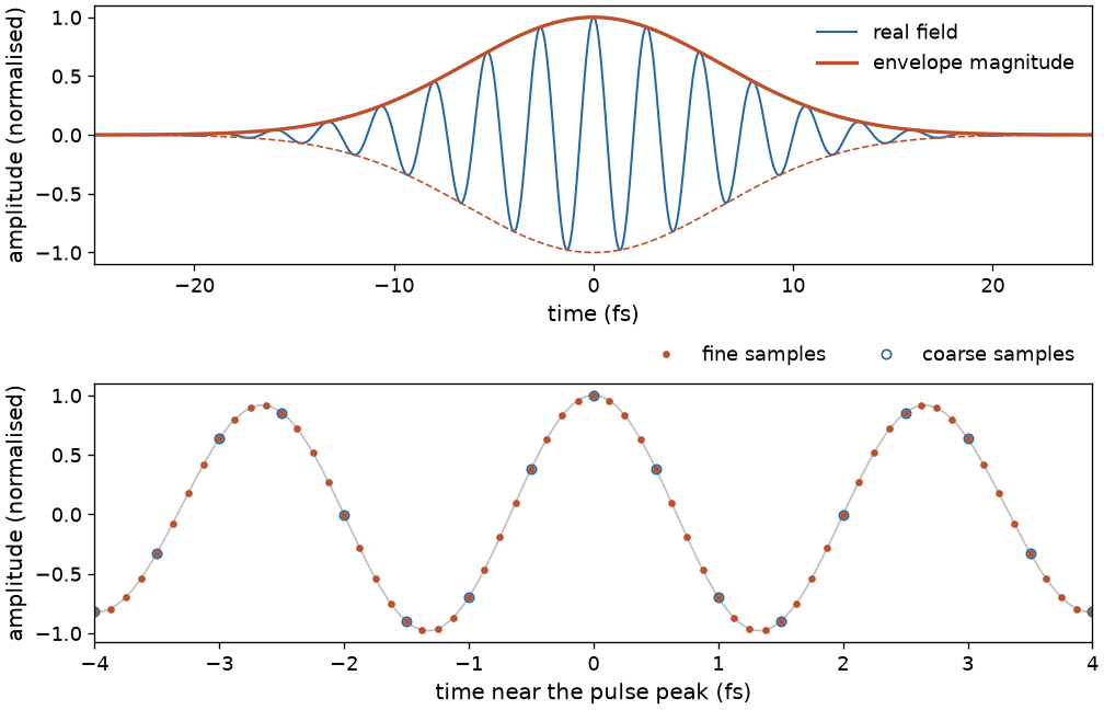
Two ways to describe a pulse, and two sampling scales within a calculation. The upper panel is an illustrative 800 nm pulse with a Gaussian amplitude envelope, not a propagated result. The lower panel shows that coarse and fine samples coincide; finer sampling is used when evaluating nonlinear responses.

	Field grid	Envelope grid
Time-domain representation	A real signal	A complex envelope
Frequency coordinates	\(\omega_k=k\,\delta\omega\), from zero to Nyquist	\(\omega=\omega_0+\nu\), where \(\nu\) is the relative frequency
Spectral samples	n_omega = n_t/2 + 1	n_omega = n_t
Ordering of the spectral array	Non-negative frequencies	FFT order: non-negative relative frequencies followed by negative ones

The stored envelope spectrum stays in FFT order: the kernels never shift it, and only processing and plotting reorder it for display.

The units of the amplitude depend on the spatial description. Guided modal amplitudes use power normalisation; free-space fields use physical field units. See power, energy and intensity.

When using the low-level functions in solprop.fourier, pass kind= explicitly. The array’s dtype does not identify its physical meaning: an unchirped envelope can be real, and a real field can be stored in a complex array.

Choose the window and wavelength range

wavelength_limits=(lambda_min, lambda_max) specifies the band of interest, in metres. trange specifies the requested time window, in seconds. The reference wavelength sets the envelope carrier and is also used in defining the moving frame. These quantities are distinct from the input pulse’s duration and spectral width.

Choose a wavelength range that contains both the input and the expected generated light. Choose a time window that contains the pulse throughout propagation, including dispersion, splitting, and the relative delay of different components. The dispersive-wave example shows why a generated pulse may move away from the pump in time.

For a realised duration \(T\) and time spacing \(\delta t\),

\[T=n_t\delta t,\qquad \delta\omega=\frac{2\pi}{T}.\]

A longer window therefore gives finer frequency spacing. Finer time sampling increases the frequency range that can be represented. These are independent requirements: improving one does not automatically resolve the other.

Start with the defaults for oversampling and transform size, then inspect the realised grid. solprop rounds sample counts to FFT-friendly sizes, so the realised window is generally different from the requested one.

from solprop.grid import FieldGrid

grid = FieldGrid.from_limits(
    length=1.5,  # propagation distance, m; no run is made here
    reference_wavelength=800e-9,  # m
    wavelength_limits=(90e-9, 4e-6),
    trange=400e-15,  # s
)
print(grid.n_t, grid.n_to, grid.n_omega)
print(f"Time window: {grid.n_t * grid.dt * 1e15:.1f} fs")

This grid has 4096 coarse time samples, 8192 fine time samples, and 2049 stored spectral samples. Its realised window is about 409.9 fs. The grid’s length is a propagation parameter; constructing it does not run a simulation.

Coarse and fine sampling

The coarse grid carries the propagated spectrum. The fine grid resolves the nonlinear response before its contribution is projected back onto that spectrum. This matters because a nonlinear operation generates higher frequencies: for example, cubing a real field produces frequency components beyond the original band. Insufficient sampling can fold those frequencies back into the band of interest, an error called aliasing.

Both time axes are centred on zero:

\[t_n=\left(n-\frac{n_t}{2}\right)\delta t,\qquad n=0,\ldots,n_t-1.\]

The sample count is even. Sizes are powers of two by default. With fft_size="smooth", even numbers whose prime factors are 2, 3, and 5 are also available. For example, a requirement of 4100 samples rounds to 8192 with the power-of-two choice and 4320 with the smooth choice.

Building a field grid

Write \(\omega_{\min}=2\pi c/\lambda_{\max}\) and \(\omega_{\max}=2\pi c/\lambda_{\min}\). The upper edge of the spectral collar is \(\omega_{\max}^{\mathrm{win}}=1.1\omega_{\max}\).

1. The fine spacing is \(\delta t_{\mathrm{fine}}=2\pi/(\mathtt{ffac}\,\omega_{\max})\), or the requested dt if that is finer. The default is ffac=6, providing sampling for the third-harmonic content of a cubic response. ffac=4 suffices for a response without that content. The allowed minimum is 2; at that minimum the upper collar is truncated rather than fully represented.

2. The fine size n_to is an allowed transform size at least trange/dt_fine. The realised duration is \(T=n_{to}\delta t_{\mathrm{fine}}\), and both grids have the same \(\delta\omega=2\pi/T\).

3. The coarse size n_t is the smallest even divisor of n_to that holds the required spectral bins through the upper collar. Its spectral size is n_omega=n_t/2+1 and \(\delta t=\pi/\omega[-1]\).

With a smooth transform, the initially rounded fine size can have too few divisors to retain the available oversampling. In that case the constructor enlarges the fine size to a compatible multiple and recomputes the two sizes. The realised window can therefore grow by more than the initial FFT rounding.

For the grid constructed above, the fine spacing is about 50.03 as. The requested 400 fs window requires about 7994 fine samples, which rounds to 8192. There are 1503 non-negative bins through the upper collar, so the coarse size rounds to 4096 and the stored half-spectrum has 2049 bins.

Important

Changing ffac can change the whole grid: its fine spacing, rounded size, realised duration, frequency spacing, and coarse size. Compare results on their common physical frequency range, with interpolation where needed; equal array indices need not represent equal frequencies.

Building an envelope grid

The envelope uses relative frequencies \(\nu=\omega-\omega_0\). Without third harmonic, the default ffac=2 gives coincident coarse and fine grids unless a finer dt is requested. With thg=True, the default is ffac=6 and the fine grid is oversampled. Without oversampling, the cubic \(|A|^2A\) is evaluated on the coarse grid itself, so its products of components near the edges of the window can fold back into it; what keeps that aliasing small is the requirement that the spectrum, with its collars, stays well inside the window. If an envelope run broadens towards the edges, check it by widening the wavelength range, not by tightening the tolerance.

The required relative span must cover both sides of the carrier:

\[\Omega=\max\left(\left|\omega_{\mathrm{hi}}-\omega_0\right|, \left|\omega_0-\tfrac12\omega_{\min}\right|\right),\]

where \(\omega_{\mathrm{hi}}=1.1\omega_{\max}\) without third harmonic and \(\omega_{\mathrm{hi}}=\omega_{\max}\) with it. The fine-spacing requirement is \(2\pi/(\mathtt{ffac}\,\Omega)\). When oversampling is used, the coarse grid still covers the active band through \(1.1\omega_{\max}\).

The lower-frequency reach matters when the carrier lies near the blue end of the band. Measuring only the upper side and applying the result to both would silently drop the low-frequency half of the band, for instance for a 100 nm reference with limits of 90 nm to 4 µm.

Matching the two time axes

The coarse size divides the fine size. With the integer ratio \(r=n_{to}/n_t\),

\[t_n=\left(n-\frac{n_t}{2}\right)r\,\delta t_{\mathrm{fine}} =\left(nr-\frac{n_{to}}{2}\right)\delta t_{\mathrm{fine}} =t^{\mathrm{fine}}_{nr}.\]

Thus every coarse sample coincides with a fine sample: t == t_fine[::r]. Selecting the coarse size from the divisors of the fine size preserves this relationship for both power-of-two and smooth transforms. It also keeps the two coarse halves of an envelope spectrum from overlapping, which would corrupt the spectrum without any error.

Oversampling: pad, evaluate, crop

A nonlinear evaluation zero-pads the coarse spectrum onto the fine grid, transforms it to time, evaluates the response, transforms back, and crops to the coarse band. Padding scales the spectrum by n_to/n_t, and cropping applies the reciprocal factor. This compensates for the different \(1/N\) factors in the inverse transforms, so coincident time samples retain the same amplitude.

For a field grid, the retained bins are the leading n_omega bins. For an envelope grid, they are the leading and trailing n_t/2 bins, representing the positive and negative relative frequencies in FFT order.

The active band and absorbing collars

Three frequency regions have different roles:

• The requested band, \([\omega_{\min},\omega_{\max}]\), is the band of interest.

• The active band, \(\omega_{\min}/2<\omega<1.1\omega_{\max}\), also includes the spectral collars. It is where dispersion and noise are evaluated and where the default stepper error norm is scored.

• Frequencies outside the active band are held at zero.

The collar profiles are smooth Planck tapers. The spectral profile rises from zero to one over \([\omega_{\min}/2,\omega_{\min}]\) and falls back to zero over \([\omega_{\max},1.1\omega_{\max}]\). A temporal collar absorbs light near each end of the time window. The boundary model explains how these profiles become absorption rates during propagation.

The temporal profile is flat for \(|t|\leq t_{\mathrm{flat}}\), where

\[t_{\mathrm{flat}}=\min\left(\frac{\mathtt{trange}}{2}, \frac{T}{2}(1-2f_c)\right),\]

and \(f_c=\mathtt{collar\_fraction}\) is 0.05 by default. Each collar therefore occupies at least that fraction of the realised window. It can extend inside the requested window when FFT rounding leaves insufficient room outside it. Inspect the collar, not just trange, when deciding whether a pulse has enough room.

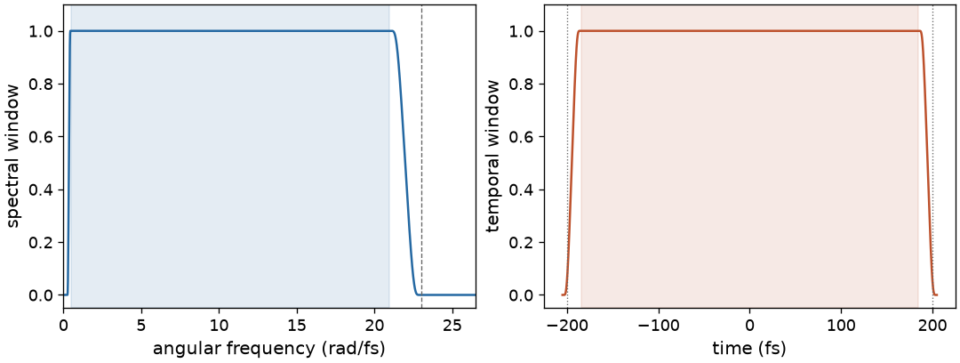
The actual collar profiles of the grid constructed in this chapter. The spectral shading marks the requested band. In time, shading marks the flat region and dotted lines mark the requested ±200 fs limits; the guaranteed collar width makes the flat region slightly smaller.

Absorbers help prevent boundary artefacts, but they remove light. If an observable changes when the window or wavelength range is enlarged, its earlier value may have been affected by the boundary. The solver chapter explains step-size control; it does not replace these grid checks.

Field-grid plasma also uses the analytic derivative of this temporal collar to hold the post-pulse current (field plasma). Translation refuses a steady-current certificate above 1e-10, naming each taper’s sample count. This is a sampling requirement on the collar, separate from the optical field absorber and from convergence with respect to the physical time window.

Fourier signs and the phase origin

User-facing spectra and phases use the optics convention,

\[\widetilde E(\omega)=\int E(t)e^{+i\omega t}\,\mathrm{d}t,\]

with a plane wave written as \(e^{i(\beta z-\omega t)}\). A delay by \(\tau\) multiplies the spectrum by \(e^{+i\omega\tau}\), and positive group-delay dispersion contributes a positive quadratic spectral phase. Saved fields and processing accessors use this convention; see input phase.

The underlying transforms use the FFT sign. Their spectra are raw forward DFTs, with no \(1/N\) or \(\delta t\) factor; the inverse transform supplies \(1/N\). There is also a phase-origin difference: a raw DFT starts at the first sample, whereas a saved optical spectrum is referenced to \(t=0\) at the centre of the time window. For both layouts the conversion is

\[\widetilde E_{\mathrm{optics},k}=(-1)^k\, \operatorname{conj}(\widetilde E_{\mathrm{internal},k}),\]

where \(k\) is the storage index. Use spectrum_to_optics() and spectrum_to_internal() for spectral arrays. They apply both the sign conversion and the origin shift. The simpler to_optics() and to_internal() perform conjugation alone and are suitable for time-domain arrays. The conversions are their own inverses.

The processing accessors handle these conventions for ordinary analysis. Use the low-level conversions when constructing a custom spectrum or working directly with raw arrays. Amplitude normalisation is a separate operation, described in power and intensity.

Energy and spectral density

For saved modal spectra, let \(B_k\) denote a power-normalised spectral amplitude on a field grid and \(A_k\) the corresponding envelope amplitude. Their discrete energies are

\[U_{\mathrm{field}}=\frac{\delta t}{n_t} \left[|B_0|^2+4\sum_{k=1}^{n_t/2-1}|B_k|^2+|B_{n_t/2}|^2\right],\]

\[U_{\mathrm{env}}=\frac{\delta t}{n_t}\sum_k|A_k|^2.\]

Sum over modes and polarisations for the total energy. These are discrete Parseval identities: the equivalent time and frequency integrals agree to round-off. The factor four in the field expression comes from doubling the interior positive-frequency amplitudes when forming the analytic signal.

The squared magnitude of the power-normalised temporal amplitude integrates to the energy, but it need not equal the temporal Poynting-flux statistic in a broadband dispersive mode. The latter includes the frequency-dependent effective index in a different way. See the definitions and interpretation before comparing a temporal trace with an intensity measurement. Spatial fields also require their transverse integration measure; these modal formulas alone do not give a free-space beam’s energy.

The spectral energy densities per angular frequency are

\[S_{\mathrm{field}}(\omega)=\frac{2\delta t^2}{\pi}|B|^2, \qquad S_{\mathrm{env}}(\omega)=\frac{\delta t^2}{2\pi}|A|^2,\]

in J/(rad/s). For a density per wavelength, apply the Jacobian \(S(\lambda)=S(\omega)\,2\pi c/\lambda^2\). Use get_spectral_density() to obtain a density in the coordinate you intend to plot. The normalisation also gives the shot-noise model one photon of energy per occupied spectral bin.

Zero frequency and Nyquist

analytic_signal() retains the zero-frequency and Nyquist bins, doubles the interior positive-frequency bins, and removes the negative ones. Retaining the endpoints makes the real part of the analytic signal recover the original real signal, following scipy.signal.hilbert().

The field spectral-density formula above uses the interior-bin prefactor. For an arbitrary array with nonzero endpoint bins, summing that density over all bins therefore differs from the exact energy formula. Use energy_omega() for exact discrete energy. Normal propagation grids suppress those endpoints through their spectral window.

Check a sampled pulse

The following continues the grid construction above. It builds a pulse without propagating it, pads and crops its spectrum, and compares its energy in both domains. GaussianPulse.build returns the internal Fourier convention, so the inverse transform can be applied directly.

import numpy as np

from solprop import fourier
from solprop.pulses import GaussianPulse

spectrum = GaussianPulse(wavelength=800e-9, fwhm=30e-15, energy=1e-6).build(grid)
fine = fourier.oversample(spectrum, grid.n_to, kind=grid.kind)
coarse = fourier.crop(fine, grid.n_t, kind=grid.kind)
energy_frequency = fourier.energy_omega(spectrum, grid.dt, kind=grid.kind)
energy_time = fourier.energy_t(
    fourier.inverse(spectrum, kind=grid.kind), grid.dt, kind=grid.kind
)
print(f"Pad/crop difference: {np.max(np.abs(coarse - spectrum)):.3e}")
print("Energy in frequency and time (J):", energy_frequency, energy_time)

Both energies are \(10^{-6}\) J, up to floating-point rounding. For an actual propagation, repeat the calculation with a wider band or time window and, where needed, finer response sampling. Compare the observables that matter for your experiment on common physical axes.

Continue with input pulses, or return to the introduction to use these choices in a complete simulation. The conventions reference records the precise interface and internal conventions for developers.