The Raman response#
A Raman-active medium remembers earlier light. A pulse can excite molecular rotation or vibration, or a delayed response in glass, which then changes the polarisation seen by later parts of the field. This memory produces effects such as Raman sidebands, frequency shifts and pulse-to-pulse coupling.
For a first calculation, use the configuration section and the comb-to-continuum example. Choose a time window that contains both the optical pulse and the response needed by your measurement. Resolving a pulse alone does not establish that a long-lived molecular coherence has been resolved.
This chapter defines the response and its regimes, then explains how to select it
in a run. Continue to the scalar models, vector response,
numerical convolution and material data for
the equations, sampling requirements and validity ranges. The underlying
molecular models assume weak excitation of an initially isotropic ensemble;
strong alignment and population redistribution need a different physical model.
The reference evaluation is in solprop.nonlinear.raman and the kernel sampling in
solprop.translate.raman. Where solprop’s choices differ from Luna.jl’s, the differences are listed in
Noteworthy differences from Luna.
The response function and its units#
For a fixed linear polarisation, the scalar reduction of an isotropic medium is
with \(\rho\) the number density in m⁻³ and \(E\) in V/m. Causality is the upper limit of the integral, and it is enforced by \(h(t) = 0\) for \(t \le 0\).
Fixing \(P\) in C/m² forces the units of \(h\): dimensionally \(\mathrm{C\,V^{-1}m^{-1}} \cdot \mathrm{m^{-3}} \cdot \mathrm{V\,m^{-1}} \cdot [h] \cdot \mathrm{V^2 m^{-2}} \cdot \mathrm{s} = \mathrm{C\,m^{-2}}\), so
and \(\int h\,dt\) carries the units of
solprop.nonlinear.responses.KerrResponse.chi3 per unit density, m⁵/V². The Kerr
and Raman strengths of the same medium are therefore directly comparable, and a Raman
fraction \(f_R\) is a plain share of the same quantity.
Note
The same physics is sometimes written without the \(\varepsilon_0\) outside the integral, with it hidden inside every scale factor as \((4\pi\varepsilon_0)^2\). An \(h\) written that way is quadratic in \(\varepsilon_0\) where solprop’s is linear, and converting such values to this convention divides by \(\varepsilon_0\).
Physical origin#
Solprop uses a deterministic, weak-excitation molecular response: the optical field perturbs an initially isotropic ensemble of molecules, and the vibration and rotation it induces change the polarisation seen by later light. The scalar molecular strengths and linewidths are sourced inputs, listed with their limitations in the data chapter. The vector extension (vector Raman) supplies only their orientation dependence; it introduces no fitted molecular constants.
The interaction energy of an induced dipole is
The half is essential: the dipole is induced, and its moment grows as the field is applied. A linear molecule with orientation \(\mathbf n\) has \(\alpha^{\rm SI}_{ij}=\bar\alpha_{\rm SI}\delta_{ij} +\Delta\alpha_{\rm SI}(n_i n_j-\delta_{ij}/3)\), with \(\bar\alpha\) the mean polarisability and \(\Delta\alpha\) its anisotropy.
Vibration. For a displacement \(q\) with effective mass \(\mu\), expanding the mean polarisability gives the driving force \(\mu\ddot q=(\partial\bar\alpha_{\rm SI}/\partial q)E^2/2\), before the restoring and damping terms. The polarisation the displacement induces contains the same derivative again, which is why the vibrational strength in the scalar models contains it squared.
Rotation. The torque couples through the anisotropy \(\Delta\alpha_{\rm SI}\) instead, and changes the orientation of the ensemble; the rotational ladder is its quantum-mechanical form.
Steady-state, transient and impulsive regimes#
There are two separate molecular clocks: the period \(2\pi/\Omega\) and the coherence decay time \(\tau_2\). In a steady-state stimulated-scattering limit, a nearly monochromatic pump–Stokes beat persists for many decay times and sets a Lorentzian gain. Transient scattering starts before that coherence has reached equilibrium; a pulse shorter than \(\tau_2\) can still contain many molecular oscillations. In the impulsive regime, the drive is short compared with a molecular period and launches a ringing response sampled by later light. Comparing pulse duration only with \(\tau_2\) does not distinguish these last two cases.
The same causal convolution can describe all three regimes within its weak excitation and material assumptions. It does not make an unresolved vibrational band into a resolved Q branch. For delayed probes, the frequency spread of unresolved rovibrational lines, spin structure and collision-partner dependence may matter earlier than the nominal single-line damping time.
Using it in a run#
A problem carries Raman when a RamanResponse is among
its responses. The drivers build that response from the material, and the three routes
below differ in their defaults. Every CPU backend (numpy_ref, numba_cpu, native) runs
it, scalar or tensor, on field and envelope grids, and the native CUDA and HIP builds are
qualified for it (backends and the drive form).
Gas fills in a capillary or waveguide#
For a gas fill in prop_capillary() or
prop_waveguide() (and the Simulation.from_capillary
and Simulation.from_waveguide constructors behind them), the raman keyword takes
|
effect |
|---|---|
|
on for every component whose optmat response is validated — H₂, D₂, N₂, O₂, CH₄ and SF₆ — as long as |
|
off |
|
every available response of the fill; the components without data are logged at INFO and left out. A single gas without data is refused by name. |
a sequence of labels, e.g. |
only those components; a label without data raises by name |
a mapping from label to |
per component, with the rotational and vibrational terms and the population temperature selected separately |
raman=True with kerr=False is refused: a medium with a Raman response has an
electronic one too, and on a field grid the drive form reaches the Raman kernel through
the Kerr term (Raman numerics). The rotational populations take
the fill’s temperature; a temperature that varies along z is reduced to one reference
value, as described under the rotational ladder. See
mixtures for the full selection vocabulary.
Air. gas="air" (in any case, or Gas.Air) on these drivers does not use the
built-in entry Gas.Air: it is expanded into Mixture.air(pressure, argon=False), a
nitrogen–oxygen mixture whose components keep their own dispersion, Kerr, plasma and
Raman channels (mixtures). Its default Raman response is therefore on,
with both the N₂ and the O₂ models. A three-component Mixture.air(...) passed as gas
behaves the same way, with argon’s omission logged. The built-in entry Gas.Air itself
is a dispersion-only species (optmat’s index of dry air as a whole): it has no Raman
data, no Kerr coefficient and no ionisation data.
Placed in a fill by hand, as in Mixture.fill({"Air": 1.0}, 1.0), it contributes no
Raman response under the default and says nothing; a run that also asks for Kerr is
refused (Air (Air) has no Kerr data), and an explicit raman=("Air",) raises. For
nonlinear propagation in air use gas="air" or Mixture.air; the
air tutorial selects the N₂
response alone with raman=("N2",).
Hand-built problems and free space#
solprop.nonlinear.mixtures.responses_for(), which builds the response list of a
free-space run or of any problem assembled by hand, has raman=False by default:
Raman is included only when asked for, with the same True, label and mapping
vocabulary as above. A single response is built by
solprop.nonlinear.raman.response_for(), which takes a built-in gas (optmat’s
response, which needs a carrier, the selection’s carrier_wavelength), a custom
Species carrying its own
MolecularRaman, or one of the silica names
("SiO2", "silica", "fused_silica", "fused silica"), and an optional
MolecularOptions:
from solprop.nonlinear.raman import MolecularOptions, response_for
from solprop.physdata import MaterialSelection

at_800nm = MaterialSelection(carrier_wavelength=800e-9)
nitrogen = response_for("N2", selection=at_800nm)  # rotation + vibration, 293.15 K
rotation = response_for("N2", MolecularOptions(vibration=False), selection=at_800nm)
silica = response_for("SiO2", fraction=0.2188)  # normalised shape, the bundle's f_R
MolecularOptions has three-state term flags: None (the default) takes a term when
the species has it, True requires it and is refused by name otherwise, False leaves
it out. Its temperature sets the rotational populations (the run’s or mixture’s own
when None, room temperature, 293.15 K, for a bare response_for), and min_j/max_j
(default 0 and 50) bound the rotational ladder. A molecular gas’s response is absolute
and is refused a fraction; silica’s is a normalised shape that needs one.
Raman in a fibre GNLSE#
prop_gnlse() and
solprop.nonlinear.gnlse.problem_from() take raman (default False) and
raman_fraction \(f_R\) (by default the silica bundle’s, 0.2188, with Raman on). With
raman=True the delayed response is fused silica’s (the scalar Hollenbeck–Cantrell
shape of the scalar models), and \(\gamma\) is
split between it and the Kerr term. The split is not the same number on both sides,
because the envelope forms differ:
in the slowly varying limit, so a Raman term of integral \(X\) acts like a Kerr term of
\(\tfrac23 X\) and carrying the whole nonlinearity needs
\(X = \tfrac32\chi^{(3)}_\text{total} = 2n_2\varepsilon_0c\), which is
raman_susceptibility(). The mapping therefore declares
response_for("SiO2", amplitude=raman_susceptibility(n2), fraction=f_R, thg=False) beside
KerrResponse(chi3=kerr_susceptibility(n2, f_R)), and
holds by construction.
With raman=False the whole of \(\gamma\) stays with the Kerr term unless raman_fraction
is given: by default no share is reserved for a response that is not there, and a
fraction given explicitly is held back so that switching Raman on adds the response to
an unchanged Kerr term. The GNLSE page sets out the rest of the
mapping. The soliton self-frequency shift on this route matches Gordon’s rate to 2.4 % at
\(T_0 = 800\) fs, among the checks in the
Raman qualification record.
Several responding species#
When several components of a fill carry a Raman response, their kernels are added
within each tensor channel (vector response)
before the shared history of the field is convolved, so a mixture costs one convolution
per channel rather than one per species. Each component’s amplitude uses its own
number density. Its linewidth, for want of partner-resolved collision data, uses the
total mixture density: an approximation, not an assertion that every collision
partner broadens alike (N₂ broadened by O₂ is not O₂ broadened by N₂). A
Component can carry its own law instead through
Component.dephasing. Every amplitude and decay rate takes part in the kernel cache’s
validity, and a change of composition reuses only the undamped kernels it leaves
unchanged. By default a mixture of built-in gases instead takes optmat’s one response
for its composition, with each pair’s curated broadening, and a pair optmat has not
curated is refused (Raman data); the per-component
responses here are a supplied species’ own.
A worked example#
Hydrogen at one amagat (about 1.09 bar at 293.15 K): optmat’s response function at an 800 nm carrier, and the gain spectrum it implies.
import matplotlib.pyplot as plt
import numpy as np

from solprop.constants import AMAGAT
from solprop.nonlinear.raman import MolecularOptions, response_for
from solprop.physdata import MaterialSelection

density = 1.0 * AMAGAT
n_to, dt = 1 << 16, 1e-15
delays = np.arange(n_to) * dt

at_800nm = MaterialSelection(carrier_wavelength=800e-9)
whole = response_for("H2", selection=at_800nm, density=density)
rotation = response_for(
    "H2", MolecularOptions(vibration=False), selection=at_800nm, density=density
)
vibration = response_for(
    "H2", MolecularOptions(rotation=False), selection=at_800nm, density=density
)

fig, (top, bottom) = plt.subplots(2, 1, figsize=(6.4, 5.0), layout="constrained")

window = delays < 1.2e-12
top.plot(1e12 * delays[window], 1e38 * whole.impulse(delays, density)[window],
         lw=0.8, color="0.2")
top.set_xlabel("delay (ps)")
top.set_ylabel(r"$h$  ($10^{-38}$ m$^5$V$^{-2}$s$^{-1}$)")
top.set_title("Raman response of hydrogen at 1 amagat, 293.15 K")

omega = 2 * np.pi * np.fft.rfftfreq(2 * n_to, dt)
for response, label in ((rotation, "rotation"), (vibration, "vibration")):
    kernel = np.zeros(2 * n_to)
    kernel[:n_to] = response.impulse(delays, density)
    gain = -np.imag(np.fft.rfft(kernel) * dt)
    band = omega < 1.1e15
    bottom.plot(1e-12 * omega[band] / (2 * np.pi), 1e26 * gain[band],
                lw=0.9, label=label)
bottom.set_xlabel("Raman shift (THz)")
bottom.set_ylabel(r"$-\mathrm{Im}\,\tilde H$  ($10^{-26}$ m$^5$V$^{-2}$)")
bottom.set_title("Stokes gain: positive where the response amplifies")
bottom.legend(frameon=False)
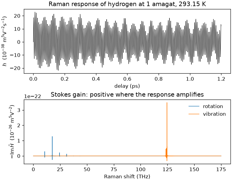
The rotational \(S(1)\) line at 17.6 THz dominates the low-frequency comb and the vibrational line sits at 124.6 THz, both with the sign that amplifies the Stokes side.
Full runs: the Raman soliton self-frequency shift in hydrogen, the Raman-comb supercontinuum and the vector Raman tutorial.