Follow vector Raman coherence with a delayed probe#

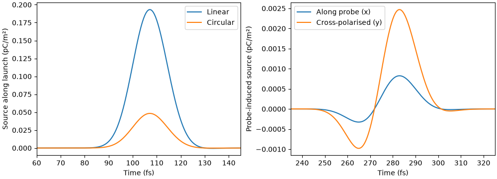
Compare equal-amplitude linear and circular envelopes using hydrogen’s rotational response. A fixed circular pump has one quarter of the rotational source along its Jones direction. This is a local polarisation comparison, not a pump-Stokes gain ratio or a propagated energy comparison.

An oblique pump also writes an off-diagonal molecular coherence. A later weak x-polarised probe acquires a y-polarised Raman source after the pump has gone. The calculation is deterministic and uses local electric fields in V/m; no spontaneous Raman noise or complex modal basis is introduced.

import matplotlib.pyplot as plt
import numpy as np

from solprop.nonlinear.raman import MolecularOptions, response_for
from solprop.physdata import MaterialSelection

spacing = 0.5e-15
time = np.arange(2048) * spacing
density = 1e25
response = response_for(
    "H2",
    MolecularOptions(vibration=False),
    selection=MaterialSelection(carrier_wavelength=800e-9),
    density=density,
)
pump = 2e8 * np.exp(-(((time - 100e-15) / 15e-15) ** 2))
probe = 0.02 * 2e8 * np.exp(-(((time - 280e-15) / 15e-15) ** 2))
linear = np.array([1.0, 0.0], complex)
circular = np.array([1.0, 1j]) / np.sqrt(2)

figure, axes = plt.subplots(1, 2, figsize=(10, 3.6), layout="constrained")
for direction, label in ((linear, "Linear"), (circular, "Circular")):
    source = response.evaluate(
        direction[:, None] * pump, density, kind="envelope", dt=spacing
    )
    along = np.real(direction.conj() @ source)
    axes[0].plot(time * 1e15, along * 1e12, label=label)
axes[0].set(xlim=(60, 145), xlabel="Time (fs)", ylabel="Source along launch (pC/m²)")
axes[0].legend()

# Subtract the pump-only response to show the weak probe's induced source.
# The pump/probe separation is large compared with their widths, so their
# instantaneous overlap is negligible. The off-diagonal history remains.
oblique = np.array([1.0, 1.0])[:, None] * pump / np.sqrt(2)
combined = oblique + linear[:, None] * probe
induced = response.evaluate(combined, density, kind="envelope", dt=spacing)
induced -= response.evaluate(
    oblique.astype(complex), density, kind="envelope", dt=spacing
)
for component, label in enumerate(("Along probe (x)", "Cross-polarised (y)")):
    axes[1].plot(time * 1e15, np.real(induced[component]) * 1e12, label=label)
axes[1].set(xlim=(235, 325), xlabel="Time (fs)", ylabel="Probe-induced source (pC/m²)")
axes[1].legend()
plt.show()

/home/docs/checkouts/solprop/checkouts/24/src/solprop/nonlinear/optmat_raman.py:1121: MaterialRangeWarning: H2: optmat's Raman response raman_response/H2@293.15K,800nm is used outside its validated density range (0.3722 to 0.3722 amagat). optmat: density below 0.94 amagat, where the motion of the molecules sets the widths: the Dicke terms are capped at the Doppler widths (TC-688)
  densities = _check_range(response, request)

Follow vector Raman coherence with a delayed probe#

Related reading#