Explore exact step-index fibres and hollow rectangular guides

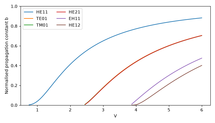
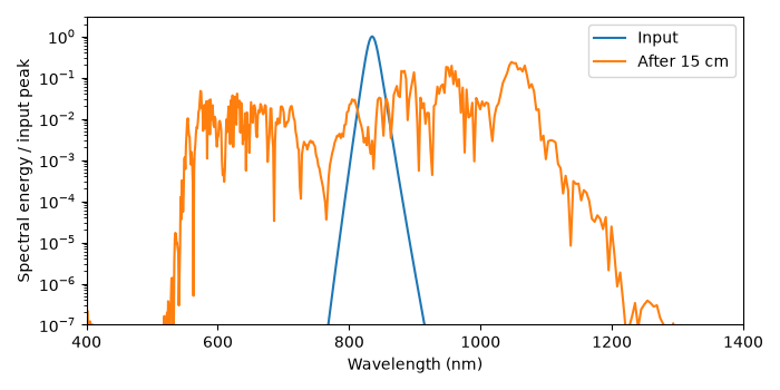
The first chart resolves the six lowest vector branches of a weakly guiding fibre: a 2 um core radius, core index 1.47 in a 1.45 cladding. Hybrid cutoffs use the exact equation; 2.405 and 3.832 are weak-guidance limits. The silica strand has a 1.25 um radius and its transverse profile is frozen at 835 nm. A 568 pJ, 50 fs sech pulse propagates for 15 cm with Kerr and silica Raman. The time window is reduced to 1 ps, and no shot noise is added. This is an example of mode-averaged propagation, not a converged supercontinuum prediction.

The strand propagates through the public prop_gnlse(fibre=...) entry: the mode supplies dispersion, loss and effective area, and n2 supplies the nonlinear response.

The rectangular comparison uses 50 by 12.5 um half-widths and both polarisation partners. Its propagation is of an aluminium-clad guide of 50 by 10 um half-widths filled with 5 bar of argon, pumped by a 30 fs pulse at 800 nm; it runs for only 1 mm with 10 nJ to keep this demonstration inexpensive. Kerr is enabled; plasma, Raman and third harmonics are disabled. The padded FFT band exceeds the argon fit and its MaterialRangeWarning is retained in the gallery output.

from time import perf_counter

import matplotlib.pyplot as plt
import numpy as np

from solprop.constants import C
from solprop.driver import prop_gnlse, prop_waveguide
from solprop.grid import EnvelopeGrid
from solprop.modes import RectMode, StepIndexMode
from solprop.modes.base import beta2, db_per_m, zdw
from solprop.physdata import aluminium, silver
from solprop.stats import StatsSpec

started = perf_counter()
figure, axis = plt.subplots(figsize=(7, 4))
for family, n, m in (
    ("HE", 1, 1),
    ("TE", 0, 1),
    ("TM", 0, 1),
    ("HE", 2, 1),
    ("EH", 1, 1),
    ("HE", 1, 2),
):
    mode = StepIndexMode(
        2e-6, core=1.47, cladding=1.45, profile_wavelength=500e-9, kind=family, n=n, m=m
    )
    v = np.linspace(max(0.75, mode.cutoff_parameter() + 0.04), 6, 80)
    omega = C * v / (2e-6 * np.sqrt(1.47**2 - 1.45**2))
    index = np.real(mode.neff(omega))
    normalised = (index**2 - 1.45**2) / (1.47**2 - 1.45**2)
    axis.plot(v, normalised, label=f"{family}{n}{m}")
axis.set(xlabel="V", ylabel="Normalised propagation constant b", ylim=(0, 1))
axis.legend(ncols=2)
figure.tight_layout()

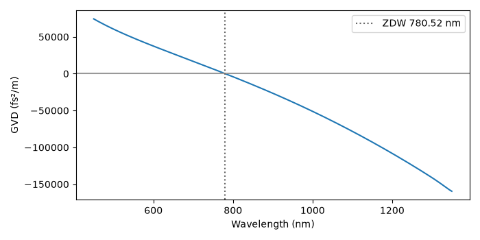
The strand dispersion and its zero crossing use the implicit derivative.

strand = StepIndexMode(1.25e-6, profile_wavelength=835e-9)
wavelength = np.linspace(450e-9, 1350e-9, 150)
zero = zdw(strand, wavelength_range=(600e-9, 900e-9))
figure, axis = plt.subplots(figsize=(7, 3.5))
axis.plot(wavelength * 1e9, beta2(strand, 2 * np.pi * C / wavelength) * 1e30)
axis.axhline(0, color="0.6")
axis.axvline(zero * 1e9, color="0.4", linestyle=":", label=f"ZDW {zero * 1e9:.2f} nm")
axis.set(xlabel="Wavelength (nm)", ylabel="GVD (fs²/m)")
axis.legend()
figure.tight_layout()

The mode itself is the fibre of a mode-averaged GNLSE run.

strand_output = prop_gnlse(
    None,
    0.15,
    fibre=strand,
    n2=2.6e-20,
    lambda0=835e-9,
    wavelength_limits=(400e-9, 1400e-9),
    trange=1e-12,
    fwhm=50e-15,
    energy=568e-12,
    pulseshape="sech",
    shock=True,
    raman=True,
    rtol=1e-5,
    atol=1e-14,
    dz_max=0.001,
    dz_init=1.5e-5,
    n_save=2,
    backend="numpy_ref",
    progress="none",
)
# The same grid prop_gnlse built from those keywords, for the wavelength axis.
grid = EnvelopeGrid.from_limits(0.15, 835e-9, (400e-9, 1400e-9), 1e-12)
figure, axis = plt.subplots(figsize=(7, 3.5))
active = grid.omega > 0
order = np.argsort(2 * np.pi * C / grid.omega[active])
spectra = np.abs(strand_output.fields("fft")[:, 0, 0, active]) ** 2
for values, label in zip(spectra, ("Input", "After 15 cm"), strict=True):
    axis.semilogy(
        (2 * np.pi * C / grid.omega[active])[order] * 1e9,
        values[order] / spectra[0].max(),
        label=label,
    )
axis.set(
    xlabel="Wavelength (nm)",
    ylabel="Spectral energy / input peak",
    xlim=(400, 1400),
    ylim=(1e-7, 3),
)
axis.legend()
figure.tight_layout()

/home/docs/checkouts/solprop/checkouts/24/src/solprop/modes/stepindex.py:572: MaterialRangeWarning: SiO2 (fit/SiO2) is taken as transparent, and drops an absorption coefficient of 2.81e+03 /m (k = 0.00061) at 2726 nm, beyond the transparent approximation's bound of 100 /m: the band reaches an absorbing region the lossless solve does not represent
  return np.asarray(np.real(lossless.index(omega))), np.asarray(

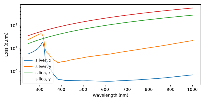
Rectangular x/y partners have separate propagation constants and losses.

wavelength = np.linspace(250e-9, 1000e-9, 250)
omega = 2 * np.pi * C / wavelength
figure, axis = plt.subplots(figsize=(7, 3.5))
for wall, name in ((silver(), "silver"), (None, "silica")):
    for polarisation in ("x", "y"):
        mode = RectMode(50e-6, 12.5e-6, cladding=wall, polarisation=polarisation)
        axis.semilogy(
            wavelength * 1e9, db_per_m(mode, omega), label=f"{name}, {polarisation}"
        )
axis.set(xlabel="Wavelength (nm)", ylabel="Loss (dB/m)")
axis.legend()
figure.tight_layout()

rectangular = prop_waveguide(
    [RectMode(50e-6, 10e-6, cladding=aluminium())],
    0.001,
    "Ar",
    5.0,
    lambda0=800e-9,
    wavelength_limits=(450e-9, 1200e-9),
    trange=100e-15,
    fwhm=30e-15,
    energy=1e-8,
    envelope=True,
    plasma=False,
    raman=False,
    n_r=12,
    n_theta=12,
    n_save=2,
    stats=StatsSpec(names=("energy",)),
    backend="numpy_ref",
    progress="none",
)
print(f"Rectangular transmitted energy: {rectangular['stats/energy'][-1].sum():.6e} J")
print(f"Complete step-index/rectangular example: {perf_counter() - started:.3f} s")

/home/docs/checkouts/solprop/checkouts/24/src/solprop/linear.py:575: GrazingIncidenceWarning: RectMode(x11, 100 um x 20 um, Ar 5 bar, loss=True): the first-order wall-pair model reaches lambda |q| / (2 pi a) = 0.179 at 2332 nm, above the 0.1 it is valid to; its neglected terms are second order in that ratio. Narrow the band towards shorter wavelengths, widen the guide, or keep lower orders
  index = np.asarray(mode.neff(omega, z))
Rectangular transmitted energy: 9.954369e-09 J
Complete step-index/rectangular example: 17.985 s

Related reading

Continue with Step-index fibres for the model, options and limits, and Assessing numerical accuracy for convergence checks. For a paced propagation lesson, return to GNLSE propagation: an N = 3 soliton.