Note
Go to the end to download the full example code.
Calibrating a weak band with the low-storage march#
LowStorageRungeKutta replays a fixed schedule
with classical RK4 in the interaction picture, holding three copies of the state where
the adaptive marches hold fifteen or more. It has no error estimate, so its accuracy is
measured from outside, on the quantity that matters, by three-level Richardson
calibration
(Fixed schedules and repeatable propagation). Here a 30 fs line beam whose peak field is
sqrt(2) times the soliton’s, twice the soliton power, self-phase modulates over one
diffraction length, and the weak band is the light
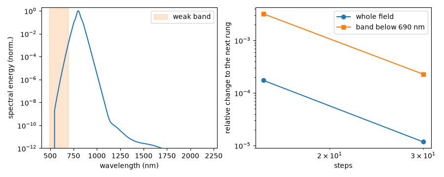
it generates below 690 nm: three parts in ten thousand of the energy. The whole field
converges twenty times faster than that band, so a norm scored on the field would call
a schedule converged while the band is still wrong. A few seconds on numpy_ref.
import itertools
import math

import matplotlib.pyplot as plt
import numpy as np

from solprop.constants import C
from solprop.driver import SimulationSettings, prop_free
from solprop.grid import EnvelopeGrid, LineGrid
from solprop.nonlinear.responses import KerrResponse
from solprop.pulses import GaussianPulse
from solprop.spatial import SpatialFlux, SpatialMedium, spatial_power
from solprop.stepper import (
    FixedSchedule,
    LowStorageRungeKutta,
    PIController,
    calibrate,
    replay,
)
A sech(x/x0) line beam whose peak field is sqrt(2) times the (1+1)-D
soliton’s, A0**2 = 8/(3 k0**2 chi3 x0**2), at the peak of a 30 fs pulse: twice
the soliton power P'. It crosses one diffraction length k x0**2 of vacuum
with an absolute Kerr susceptibility (the line tutorial’s beam, shorter and
stronger). The temporal envelope has unit peak, so the field is stated directly.
wavelength, chi3, x0 = 800e-9, 3e-26, 50e-6
k0 = 2 * math.pi / wavelength
amplitude = math.sqrt(2 * 8 / (3 * k0**2 * chi3 * x0**2))  # V/m
length = k0 * x0**2
space = LineGrid(20 * x0, 64, window_factor=0)
grid = EnvelopeGrid.from_limits(
    length, wavelength, (600e-9, 1.1e-6), 400e-15, thg=False
)
vacuum = SpatialMedium()
flux = SpatialFlux.resolve(grid, space, vacuum)
profile = 1 / np.cosh(space.x / x0)
envelope = GaussianPulse(wavelength=wavelength, fwhm=30e-15, peak_power=1.0).build(grid)
start = amplitude * np.fft.fft(profile)[:, None, None] * envelope
print(f"peak power {np.max(spatial_power(start, flux)):.4g} W/m, 2 P'")
band = (2 * math.pi * C / grid.omega < 690e-9) & grid.active_mask
# Each column's energy weight is its real axial admittance in vacuum, the obliquity.
weight = space.spectral_weights[:, None] * np.real(flux.admittance())


def replayed(schedule, mode="auto"):
    """Replay `schedule` with the low-storage march; return the final spectra."""
    settings = SimulationSettings(
        controller=PIController(rtol=1e-6, atol=1e-12),
        save_planes=[length],
        dz_init=schedule.max_step,
        dz_max=schedule.max_step,
        schedule=schedule,
        integrator=LowStorageRungeKutta(),
        propagator_mode=mode,
    )
    result = prop_free(
        grid,
        space,
        vacuum,
        [KerrResponse(chi3, thg=False)],
        start,
        settings=settings,
    )
    return result.fields("fft")[1]


def band_fraction(field):
    """Return the energy fraction below 690 nm, summed over the line."""
    spectrum = np.sum(weight * np.sum(np.abs(field) ** 2, axis=1), axis=0)
    return float(spectrum[band].sum() / spectrum.sum())
peak power 1.53e+14 W/m, 2 P'
The parity floor: two computations of one schedule that differ by rounding alone
measure how far down the band can be resolved at all. While numpy_ref is the one
backend executing the march, its two flow treatments – one tabulated half-step flow
reused across steps, or the flow formed in every pass – are those two computations.
band fraction 3.384e-04, parity floor 0.0e+00
Three levels, 15, 30 and 60 steps: the observed order and the error the base schedule
actually carries, extrapolated. order=4 arms the gate that refuses an order above
seven; requested is only quoted, since no adaptive run discovered this schedule.
fields = {}


def observable(schedule):
    """Replay a rung, keep its field, and return the band fraction."""
    fields[schedule.n_steps] = replayed(schedule)
    return band_fraction(fields[schedule.n_steps])


calibration = calibrate(base, observable, order=4, requested=1e-6, floor=floor)
print(calibration.message)
observed order 3.81 against a stated order of 4; achieved error 1.17e-06 for a requested tolerance of 1.00e-06
The whole field against the band, rung by rung: the field’s relative change is what a norm scored on the whole state sees, and it is twenty times smaller than the band’s.
rungs = sorted(fields)
field_change = [
    float(np.linalg.norm(fields[a] - fields[b]) / np.linalg.norm(fields[b]))
    for a, b in itertools.pairwise(rungs)
]
band_change = [
    abs(band_fraction(fields[a]) - band_fraction(fields[b])) / band_fraction(fields[b])
    for a, b in itertools.pairwise(rungs)
]
for (a, b), whole, weak in zip(
    itertools.pairwise(rungs), field_change, band_change, strict=True
):
    print(f"{a} -> {b} steps: field {whole:.1e}, band {weak:.1e}")
15 -> 30 steps: field 1.7e-04, band 3.2e-03
30 -> 60 steps: field 1.2e-05, band 2.3e-04
Replay to a target: one part in a thousand of the band. The schedule is rescaled along the measured exponent, and the production run’s band is compared with the finest rung.
21 steps; band 3.392787e-04 against the finest rung's 3.395941e-04
The final spectral energy, summed over the line, with the weak band shaded.
spectrum = np.sum(weight * np.sum(np.abs(fields[rungs[-1]]) ** 2, axis=1), axis=0)
order = np.argsort(grid.omega)
wavelengths = 2 * math.pi * C / grid.omega[order] * 1e9
figure, (left, right) = plt.subplots(1, 2, figsize=(9, 3.6))
left.semilogy(wavelengths, spectrum[order] / spectrum.max(), "C0")
left.axvspan(wavelengths.min(), 690, color="C1", alpha=0.2, label="weak band")
left.set(xlabel="wavelength (nm)", ylabel="spectral energy (norm.)", ylim=(1e-12, 2))
left.legend()
right.loglog(rungs[:-1], field_change, "o-", label="whole field")
right.loglog(rungs[:-1], band_change, "s-", label="band below 690 nm")
right.set(xlabel="steps", ylabel="relative change to the next rung")
right.legend()
figure.tight_layout()