Supercontinuum by modulational instability

Modulational instability (MI) amplifies small perturbations on a pulse through the combined action of Kerr nonlinearity and anomalous dispersion. A long pulse can break into shorter structures whose spectra broaden differently in each shot. An average spectrum can therefore look smooth even when individual spectra vary strongly. This example separates these two observations: spectral broadening and shot-to-shot reproducibility.

We launch a 400 fs, 5 uJ pulse at 1030 nm into 0.4 m of argon-filled capillary, with core radius 16 um and pressure 40 bar. The high pressure puts the zero-dispersion wavelength at about 877 nm, below the pump, so the pump sees weak anomalous dispersion (\(\beta_2 \approx -520\) fs²/m) and strong Kerr nonlinearity: the conditions for noise-driven MI. Eight calculations retain the same pulse and material parameters and change only the seed of the input quantum noise. The propagation uses mode averaging: the fundamental mode’s effective area determines the nonlinear strength, with no transverse quadrature or modal conversion. This is a different approximation from resolving the nonlinear polarisation across a single transverse mode.

Dispersion, instantaneous Kerr nonlinearity and photoionisation are included. Argon has no molecular Raman response. Waveguide loss is disabled to isolate the nonlinear dynamics; this does not supply the dispersion or resonance structure of a particular antiresonant fibre. The broad computational band extends beyond some material fits’ validated ranges. Warnings about those ranges are suppressed below, but the extrapolated parts of the spectrum need corresponding caution.

Read the spectral map first, then compare the individual exit spectra with their mean. Relative intensity noise (RIN) measures fluctuations of spectral intensity; first-order coherence measures reproducibility of the complex field. Eight shots illustrate these distinctions but do not provide a converged ensemble estimate: the coherence of independent fields estimated from \(N\) shots scatters about zero with a spread of order \(1/\sqrt{N}\), about 0.35 here. In weak spectral wings either estimate is especially sensitive to sampling and noise. A single realisation cannot establish coherence.

For the spatial approximation see Spatial decompositions; for the noise convention and estimator see Shot noise and Processing: reading a run back. The introductory Resonant dispersive-wave propagation follows a shorter pulse whose broadening is organised by self-compression and dispersive-wave emission.

The ensemble

Each shot is the same run with a different realisation of the quantum shot noise: one photon per active spectral bin, with a random phase, added to the input spectrum (noise="input"), drawn from the generator seeded by seed. Clearing the transverse quadrature selects mode averaging. Merely setting modes=1 would retain a resolved single-mode calculation. The assertions check both the translated problem and the saved metadata so the approximation is recorded with the result.

import time
import warnings
from dataclasses import replace

import matplotlib.pyplot as plt
import numpy as np

from solprop.constants import C
from solprop.driver import Simulation
from solprop.exceptions import MaterialRangeWarning
from solprop.processing import g12_of, get_spectral_density
from solprop.stats import default_spec

SHOTS = 8
"""The size of the ensemble."""

started = time.perf_counter()
runs = []
with warnings.catch_warnings():
    warnings.simplefilter("ignore", MaterialRangeWarning)
    for seed in range(SHOTS):
        simulation = Simulation.from_capillary(
            16e-6,
            0.4,
            "Ar",
            40.0,
            lambda0=1030e-9,
            fwhm=400e-15,
            energy=5e-6,
            loss=False,
            plasma=True,
            raman=False,
            trange=4e-12,
            wavelength_limits=(170e-9, 4e-6),
            noise="input",
            seed=seed,
            n_save=101,
        )
        simulation.settings = replace(
            simulation.settings,
            quadrature=None,
            components=None,
            stats=default_spec("mode_averaged"),
        )
        assert simulation.translate().flags.mode_averaged
        run = simulation.run(progress="none")
        assert run.metadata.simulation_kind == "mode_averaged"
        assert run.metadata.quadrature is None
        runs.append(run)
        print(f"seed {seed}: {run.metadata.simulation_kind}, z = {run['z'][-1]:.2f} m")

seed 0: mode_averaged, z = 0.40 m
seed 1: mode_averaged, z = 0.40 m
seed 2: mode_averaged, z = 0.40 m
seed 3: mode_averaged, z = 0.40 m
seed 4: mode_averaged, z = 0.40 m
seed 5: mode_averaged, z = 0.40 m
seed 6: mode_averaged, z = 0.40 m
seed 7: mode_averaged, z = 0.40 m

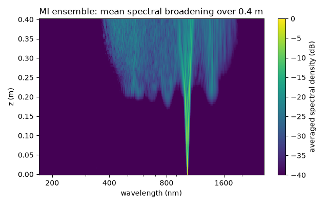
The averaged spectrum along the fibre

The spectral energy density averaged over the ensemble, in decibels below its peak.

z = np.asarray(runs[0]["z"])
spectra = []
for run in runs:
    wavelength, density = get_spectral_density(run, "wavelength")
    spectra.append(density)
spectra = np.asarray(spectra)  # (shots, planes, wavelengths)
mean = spectra.mean(axis=0)
shown = (wavelength > 170e-9) & (wavelength < 2.6e-6)
ticks = [200, 400, 800, 1600]  # nm, labelled in full on the log axis

fig, ax = plt.subplots(figsize=(6.4, 4.0))
ax.set_title("MI ensemble: mean spectral broadening over 0.4 m")
image = ax.pcolormesh(
    wavelength[shown] * 1e9,
    z,
    10 * np.log10(np.maximum(mean[:, shown] / mean.max(), 1e-12)),
    vmin=-40,
    vmax=0,
    shading="auto",
)
ax.set_xscale("log")
ax.set_xticks(ticks, labels=[str(tick) for tick in ticks])
ax.tick_params(axis="x", which="minor", labelbottom=False)
ax.set_xlabel("wavelength (nm)")
ax.set_ylabel("z (m)")
fig.colorbar(image, ax=ax, label="averaged spectral density (dB)")
fig.tight_layout()

Noise and coherence at the exit

From top to bottom: the exit spectra of every shot (grey) and their mean (black); the relative intensity noise, the standard deviation of the spectral density over its mean, shot to shot; and the first-order coherence \(|g_{12}^{(1)}(\lambda)|\) of the ensemble’s complex spectra (0 for independent fields, 1 for identical ones).

exit_mean = spectra[:, -1].mean(axis=0)
rin = np.divide(
    spectra[:, -1].std(axis=0),
    exit_mean,
    out=np.zeros_like(exit_mean),
    where=exit_mean > 0,
)
omega, coherence = g12_of(runs, plane=-1)
coherent_wavelength = 2 * np.pi * C / omega
significant = exit_mean > 1e-4 * exit_mean[shown].max()

fig, (top, middle, bottom) = plt.subplots(3, 1, figsize=(6.4, 7.5), sharex=True)
fig.suptitle("Eight exit spectra, intensity noise and field coherence")
for shot in spectra[:, -1]:
    top.semilogy(wavelength[shown] * 1e9, shot[shown], color="0.75", linewidth=0.5)
top.semilogy(wavelength[shown] * 1e9, exit_mean[shown], color="k", linewidth=1.0)
top.set_ylim(1e-6 * exit_mean[shown].max(), 3 * exit_mean[shown].max())
top.set_ylabel("spectral density (J/m)")
keep = shown & significant
middle.semilogy(wavelength[keep] * 1e9, rin[keep], color="tab:red", linewidth=1.0)
middle.set_ylabel("RIN")
in_window = (coherent_wavelength > 170e-9) & (coherent_wavelength < 2.6e-6)
bottom.plot(
    coherent_wavelength[in_window] * 1e9, coherence[in_window], color="tab:blue"
)
bottom.set_ylim(0, 1.05)
bottom.set_ylabel("coherence $|g_{12}|$")
bottom.set_xscale("log")
bottom.set_xticks(ticks, labels=[str(tick) for tick in ticks])
bottom.tick_params(axis="x", which="minor", labelbottom=False)
bottom.set_xlabel("wavelength (nm)")
fig.tight_layout()

# The estimators above are resolved in wavelength. A summary weighted by energy
# would also need each wavelength bin's width: the Fourier grid is uniform in
# frequency, not in wavelength. We retain the curves so narrow coherent features
# are not hidden by a single average.

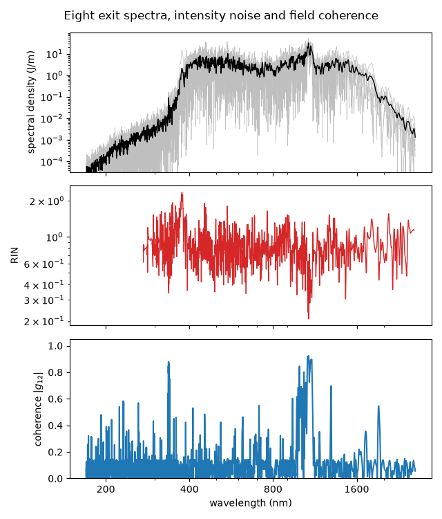
In this 0.4 m calculation, broadening becomes pronounced around 0.2 m on the displayed 40 dB scale. The exit spectrum spans the visible and near infrared, with substantial differences between shots. RIN is of order unity over much of the continuum; coherence is low over broad regions, with a more reproducible remnant near the pump. Isolated coherence peaks should not be overinterpreted with only eight shots.

Runtime and further checks

Repeat with more seeds before using these curves as quantitative ensemble statistics. Check temporal sampling and band limits independently of the propagation tolerance; see Grids and Fourier conventions.

print(
    f"{time.perf_counter() - started:.0f} s for {len(runs)} shots; "
    f"backend {runs[0].metadata.backend.name}"
)

620 s for 8 shots; backend native