Inspect step-index and graded-index electric fields#

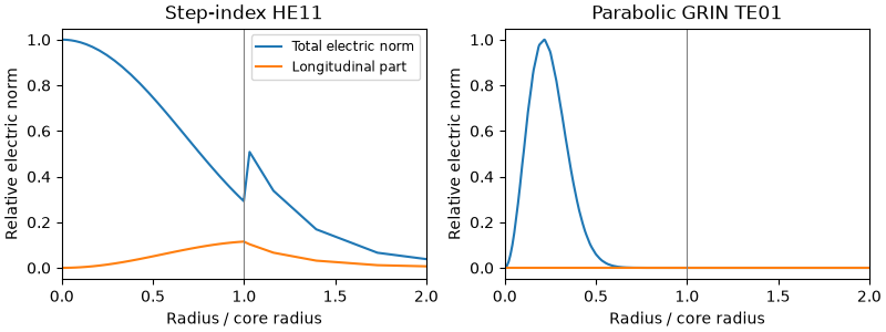
Compare a bound hybrid strand mode with a radial TE graded-index mode. The providers return full E/H fields normalised by Poynting flux. This example inspects mode construction; to propagate on such a guide, pass it to prop_waveguide(provider=...) (the general modal route: see Propagate a vector fibre mode, and check it against the GNLSE, Self-imaging in a graded-index guide, and a launch declared as a field and the worked examples).

import matplotlib.pyplot as plt
import numpy as np

from solprop.constants import C
from solprop.modes import (
    GradedIndexProvider,
    IndexMaterial,
    ModalGuide,
    PowerLawPermittivity,
    StepIndexMode,
)

omega = 2 * np.pi * C / 835e-9
mode = StepIndexMode(250e-9, core=1.45, cladding=1.0, profile_wavelength=835e-9)
step = ModalGuide.from_step_index(
    [mode], core=IndexMaterial(1.45), cladding=IndexMaterial(1.0)
).field_provider
step_nodes = step.node_rule(omega, n_r=32, n_theta=9)
step_fields = step.solve(omega, 0.0, nodes=step_nodes)
grin = GradedIndexProvider(
    permittivity=PowerLawPermittivity(IndexMaterial(1.45), 0.005),
    exterior=IndexMaterial(1.45 * np.sqrt(0.99)),
    radius=25e-6,
    family="TE",
    count=1,
    elements=32,
    extent=2.0,
)
grin_nodes = grin.node_rule(2 * np.pi * C / 1.03e-6, n_theta=9)
grin_fields = grin.solve(2 * np.pi * C / 1.03e-6, 0.0, nodes=grin_nodes)

fig, axes = plt.subplots(1, 2, figsize=(8, 3), constrained_layout=True)
for ax, nodes, sample, radius, title in (
    (axes[0], step_nodes, step_fields, 250e-9, "Step-index HE11"),
    (axes[1], grin_nodes, grin_fields, 25e-6, "Parabolic GRIN TE01"),
):
    # The polar rule lays its nodes out angle-major, so the layout is
    # (n_theta, n_radial). Take n_theta from the rule that built it rather than
    # writing the number in twice.
    n_theta = nodes.identity["n_theta"]
    radial = np.hypot(nodes.xy[:, 0], nodes.xy[:, 1]).reshape(n_theta, -1)[0] / radius
    electric = (
        np.sum(abs(sample.electric[:, :, 0]) ** 2, axis=1)
        .reshape(n_theta, -1)
        .mean(axis=0)
    )
    longitudinal = abs(sample.electric[:, 2, 0]) ** 2
    longitudinal = longitudinal.reshape(n_theta, -1).mean(axis=0)
    ax.plot(radial, electric / electric.max(), label="Total electric norm")
    ax.plot(radial, longitudinal / electric.max(), label="Longitudinal part")
    ax.axvline(1, color="grey", linewidth=0.8)
    ax.set(
        xlim=(0, 2),
        xlabel="Radius / core radius",
        ylabel="Relative electric norm",
        title=title,
    )
axes[0].legend(fontsize="small")
plt.show()

Inspect step-index and graded-index electric fields#

Related reading#