Soliton self-compression and ultraviolet dispersive-wave emission

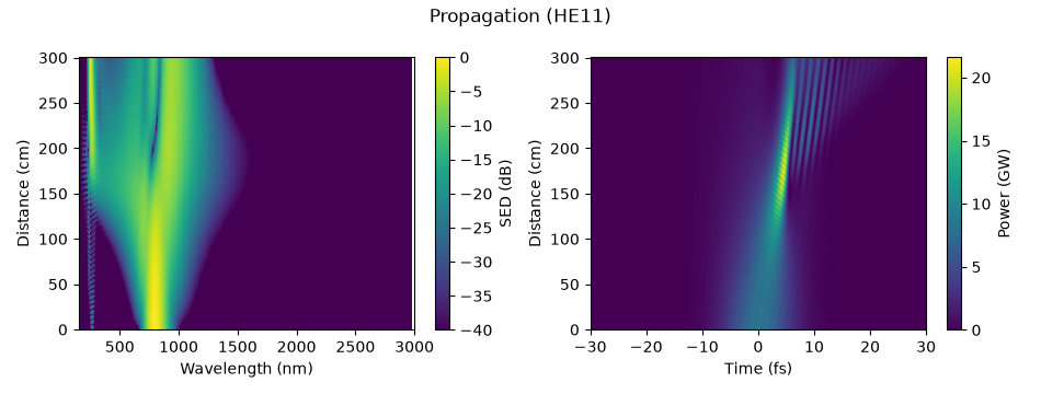
When the dispersion of the gas-filled waveguide is anomalous at the pump wavelength, the spectral phase that self-phase modulation writes is compensated as it is written: the blue-shifted trailing edge catches up with the red-shifted leading edge, the pulse gets shorter, its peak power rises, the nonlinearity grows, and the pulse can undergo strong compression. Higher dispersion, loss, ionisation and departure from the ideal NLSE alter that evolution. This is soliton self-compression, the dynamics of a higher-order soliton of order \(N = \sqrt{L_D/L_{NL}}\) in the language of the nonlinear Schrödinger equation. In a gas-filled capillary the anomalous dispersion comes from the waveguide and is smooth over a huge bandwidth, so the compression can continue to a single optical cycle and below.

At the point of maximum compression the spectrum reaches far enough into the ultraviolet to overlap a phase-matched resonant dispersive wave: linear waves at the wavelength where the mode’s dispersion matches the soliton’s effective propagation wavenumber grow from the compressed pulse and then separate from it. With helium at 2 bar in a 125 um capillary the resonance lies near 260 nm; lower pressures move it into the vacuum ultraviolet (see the first example of this gallery).

The parameters are those of high-energy soliton self-compression (HISOL): a 10 fs, 88 uJ pulse at 800 nm in 3 m of capillary with a 125 um core radius, filled with helium at 2 bar – a soliton of order about 2, in a fibre about one dispersion length long.

What to look for. In time, the pulse shortens steadily and reaches its shortest, a few femtoseconds, before the end of the fibre; at that point a narrow band appears in the deep ultraviolet and a weak trailing structure forms behind the pulse in time. The line plot compares the input with the pulse at the plane of maximum compression.

What is approximate. Only the fundamental mode is carried; the Marcatili loss of the capillary is an approximation in the deep ultraviolet.

This is panel (b) of the survey of nonlinear processes in the review by Travers et al.; the physics is described in J. C. Travers, T. F. Grigorova, C. Brahms and F. Belli, “High-energy pulse self-compression and ultraviolet generation through soliton dynamics in hollow capillary fibres”, Nature Photonics 13, 547-554 (2019).

The N = 3 soliton lesson isolates compression and recurrence in the ideal NLSE limit. Compare it with the RDW lesson for a broadband gas-filled guide.

The run

import time

import matplotlib.pyplot as plt
import numpy as np

from solprop.driver import prop_capillary
from solprop.plotting import prop_2d, spec_1d, time_1d
from solprop.processing import bandpass, energy, fwhm_t, grid_of, peak_power

started = time.perf_counter()
run = prop_capillary(
    125e-6,
    3.0,
    "He",
    2.0,
    lambda0=800e-9,
    fwhm=10e-15,
    energy=88e-6,
    trange=400e-15,
    wavelength_limits=(130e-9, 4e-6),
    n_save=301,
    progress="none",
)

Spectral and temporal evolution

figures = prop_2d(
    run,
    "wavelength",
    wavelength_range=(150e-9, 3e-6),
    trange=(-30e-15, 30e-15),
    db_min=-40,
)
figures[-1].set_size_inches(9.5, 3.6)
figures[-1].tight_layout()

Maximum compression

The plane of highest peak power, and the pulse there against the input.

z = np.asarray(run["z"])
peaks = np.asarray(peak_power(run))
best = int(np.argmax(peaks))
width = fwhm_t(run, plane=best) * 1e15
print(
    f"maximum compression at z = {z[best]:.2f} m: {width:.2f} fs FWHM, "
    f"{peaks[best] * 1e-9:.1f} GW (input {peaks[0] * 1e-9:.1f} GW)"
)

fig, (left, right) = plt.subplots(1, 2, figsize=(10.0, 3.6))
time_1d(run, z=[0.0, float(z[best])], trange=(-30e-15, 30e-15), ax=left)
spec_1d(run, z=[0.0, float(z[best]), 3.0], ax=right, wavelength_range=(150e-9, 1.5e-6))
fig.tight_layout()

uv = bandpass(grid_of(run), (200e-9, 320e-9))
uv_energy = float(np.sum(energy(run, plane=-1, bandpass=uv)))
print(f"200-320 nm at the exit: {uv_energy * 1e6:.2f} uJ")

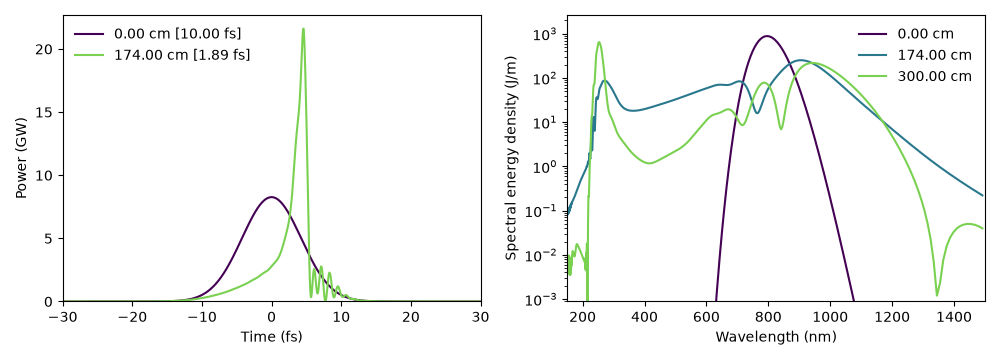
maximum compression at z = 1.74 m: 1.90 fs FWHM, 21.5 GW (input 8.3 GW)
200-320 nm at the exit: 14.00 uJ

Runtime and reproducibility

print(f"{time.perf_counter() - started:.0f} s; backend {run.metadata.backend.name}")

10 s; backend native