Note
Go to the end to download the full example code.
A planar guide resolved in y#
The hybrid planar transform: the slab modes of a 127 um argon-filled gap (Akturk et
al. 2009) in x, and a periodic, collared y axis. Unlike the slab uniform in y of
A hollow planar waveguide, per unit width, the beam here has a
finite height, so the run integrates over y and reports energy in J, and the model can
describe
diffraction, whole-beam self-focusing and modulational instability in y,
subject to the retained modes, grid, boundary and response assumptions. A 1 mJ, 100 fs
pulse (the incident beam’s physical energy in the argon fill),
Gaussian in both directions (w_x = 0.735a projected onto TE1, TE3 and TE5;
w_y = 0.5 mm), propagates 10 cm with the Kerr effect under the step controller;
the run takes seconds on numpy_ref, the reference backend. numba_cpu and the
native backend execute the geometry too.
from time import perf_counter

import matplotlib.pyplot as plt
import numpy as np

from solprop.boundaries import absorber
from solprop.driver import SimulationSettings, prop_planar
from solprop.grid import EnvelopeGrid
from solprop.modes import PlanarGrid, SlabMode
from solprop.nonlinear.responses import KerrResponse
from solprop.physdata import gamma3
from solprop.pulses import GaussianPulse, PlanarPulse
from solprop.spatial import (
    SpatialFlux,
    SpatialMedium,
    planar_fluence,
    planar_mode_energy,
)
from solprop.stats import default_spec
from solprop.stepper import PIController

started = perf_counter()
half_gap, length = 63.5e-6, 0.1
The grid carries the slab channels, their rule in x and the y axis with its absorbing collar; the launch projects its x profile onto the modes, with signs, and its energy is the incident beam’s, measured in the fill, so the modes carry the coupled share. Each mode’s energy uses the slab metric, whose weight at k_y = 0 is the mode’s real effective index (Energy and flux in a medium).
grid = EnvelopeGrid.from_limits(length, 800e-9, (650e-9, 1000e-9), 400e-15)
modes = [SlabMode(half_gap, "Ar", 1.0, order=p) for p in (1, 3, 5)]
space = PlanarGrid(modes, 1.5e-3, 64)
launch = PlanarPulse(
    GaussianPulse(wavelength=800e-9, fwhm=100e-15, energy=1e-3),
    0.5e-3,
    waist_x=0.735 * half_gap,
)
print(space)
PlanarGrid: slab modes in x, periodic samples in y
  modes:           TE1, TE3, TE5
  gap:             127 um
  x nodes:         37 (slab rule)
  half-width in y: 1.5 mm, 64 samples
  spacing in y:    51.56 um
  window factor:   0.1
  measure:         area: energy J, power W
The Kerr effect of argon, whose per-particle hyperpolarisability the run scales by the fill’s density. The collar absorbs whatever reaches it. Its damping is integrated explicitly in every nonlinear stage, so a step longer than about 7 mm here is unstable (The free-space model): the step controller’s error estimate keeps its steps below that, while a fixed schedule of ten 1 cm steps would be refused at translation.
settings = SimulationSettings(
    controller=PIController(rtol=1e-3, atol=1e-9),
    save_planes=[length],
    dz_max=length / 10,
    dz_init=1e-3,
    absorber=absorber(grid, boundary_length=1.0),
    stats=default_spec("free"),
    backend="numpy_ref",
)
output = prop_planar(
    grid,
    space,
    [KerrResponse(gamma3("Ar", wavelength=800e-9), thg=False)],
    launch,
    settings=settings,
    progress="none",
)
first, last = output.fields("fft")
fill = SpatialMedium("Ar", pressure=1.0)  # the slab modes' own fill
entrance = SpatialFlux.resolve(grid, space, fill)
exit_plane = SpatialFlux.resolve(grid, space, fill, z=length)
energy = np.ravel(output["stats/energy"])
print(f"energy {energy[0] * 1e3:.4f} mJ -> {energy[-1] * 1e3:.4f} mJ")
for mode, value in zip(modes, planar_mode_energy(last, exit_plane), strict=True):
    print(f"  {mode.channel_label.display_label}: {value * 1e3:.5f} mJ")
energy 0.9902 mJ -> 0.9607 mJ
  TE1: 0.95946 mJ
  TE3: 0.00066 mJ
  TE5: 0.00055 mJ
The fluence, the time-integrated axial flux, at the exit on the rule’s (x, y) nodes,
and across y after integrating over the gap. The widths in y are the run’s
beam_radius statistic.
fluence = planar_fluence(last, exit_plane).reshape(space.n_y, space.x.size)
figure, (section, profile) = plt.subplots(1, 2, figsize=(9, 3.6))
section.pcolormesh(space.x * 1e6, space.y * 1e3, fluence * 1e-4, shading="nearest")
section.set(xlabel="x (um)", ylabel="y (mm)", title="exit fluence (J/cm²)")
for label, plane, flux in (("entrance", first, entrance), ("exit", last, exit_plane)):
    across = planar_fluence(plane, flux).reshape(space.n_y, -1) @ space.x_weights
    profile.plot(space.y * 1e3, across, label=label)
profile.set(xlabel="y (mm)", ylabel="fluence across the gap (J/m)")
profile.legend()
figure.tight_layout()
radius = np.ravel(output["stats/beam_radius"])[-1]
print(f"1/e^2 half-width in y at the exit: {radius * 1e3:.3f} mm")
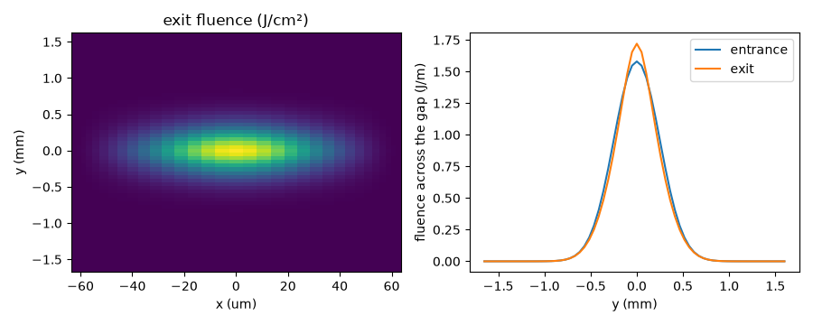
1/e^2 half-width in y at the exit: 0.475 mm
print(f"ran in {perf_counter() - started:.1f} s on numpy_ref")
ran in 3.3 s on numpy_ref