A line beam: diffraction and the (1+1)-D Kerr soliton#

A LineGrid propagates a beam that is uniform in y, per metre of y: free space resolved in x alone. Its energies are in J/m and its powers in W/m. With one free transverse dimension Kerr self-focusing does not collapse; the stationary beam is the soliton A0 sech(x/x0), whose peak field obeys A0**2 = 8 / (3 k0**2 chi3 x0**2) whatever its width. Its physical power per metre of y is then 8 n0 eps0 c / (3 k0**2 chi3 x0) (The free-space model). Here a long pulse carries that field at its peak through three diffraction lengths in vacuum with an absolute Kerr susceptibility, and at half the power, a field lower by sqrt(2), the same beam diffracts. Ten fixed steps each; the run takes seconds.

import math

import matplotlib.pyplot as plt
import numpy as np

from solprop.driver import SimulationSettings, prop_free
from solprop.exceptions import GridError
from solprop.grid import EnvelopeGrid, LineGrid
from solprop.nonlinear.responses import KerrResponse
from solprop.pulses import GaussianPulse
from solprop.spatial import (
    SpatialFlux,
    SpatialMedium,
    critical_power,
    spatial_energy,
    spatial_intensity,
    spatial_power,
)
from solprop.stepper import FixedSchedule, PIController

The soliton’s peak field, and the line. A critical power has no meaning here, and asking for one on a line is refused by name.

wavelength, chi3, x0 = 800e-9, 3e-26, 50e-6
k0 = 2 * math.pi / wavelength
amplitude = math.sqrt(8 / (3 * k0**2 * chi3 * x0**2))  # V/m
length = 3 * k0 * x0**2
space = LineGrid(20 * x0, 128, window_factor=0)
print(f"soliton peak field {amplitude:.4g} V/m; 3 diffraction lengths {length:.3g} m")
try:
    critical_power(wavelength, chi3, index=1.0, space=space)
except GridError as error:
    print(f"refused: {str(error)[:72]}...")

soliton peak field 2.401e+10 V/m; 3 diffraction lengths 0.0589 m
refused: critical_power does not apply to a LineGrid: a beam uniform in y has one...

A long pulse whose peak carries the soliton field A0 sech(x/x0) (or 1/sqrt(2) of it): the transverse profile times a temporal envelope of unit peak. Its power per metre of y, the axial Poynting flux through the entrance plane, is measured from the field rather than assumed.

grid = EnvelopeGrid.from_limits(length, wavelength, (770e-9, 832e-9), 3e-12, thg=False)
vacuum = SpatialMedium()
flux = SpatialFlux.resolve(grid, space, vacuum)
profile = 1 / np.cosh(space.x / x0)
spectrum = np.fft.fft(profile)
envelope = GaussianPulse(wavelength=wavelength, fwhm=500e-15, peak_power=1.0).build(
    grid
)
settings = SimulationSettings(
    controller=PIController(rtol=1e-8, atol=1e-14),
    save_planes=[length],
    dz_init=length / 10,
    dz_max=length,
    schedule=FixedSchedule.uniform(0.0, length, length / 10),
    backend="numpy_ref",
)
figure, axis = plt.subplots(figsize=(6, 4))
for fraction, colour in ((1.0, "C0"), (0.5, "C1")):
    start = math.sqrt(fraction) * amplitude * spectrum[:, None, None] * envelope
    power = float(np.max(spatial_power(start, flux)))
    result = prop_free(
        grid,
        space,
        vacuum,
        [KerrResponse(chi3, thg=False)],
        start,
        settings=settings,
    )
    first, last = result.fields("fft")
    before = spatial_intensity(first, flux)
    after = spatial_intensity(last, flux)
    peak = float(np.max(before))
    column = int(np.argmax(np.max(after, axis=0)))
    axis.plot(
        space.x * 1e6,
        after[:, column] / peak,
        colour,
        label=f"{fraction:g} P' after 3 k x0²",
    )
    print(
        f"{fraction:g} P': peak power {power:.4g} W/m, "
        f"energy {spatial_energy(last, flux):.4g} J/m, "
        f"peak intensity ratio {np.max(after) / peak:.4f}"
    )
axis.plot(space.x * 1e6, profile**2, "k--", label="sech²(x/x0), launched")
axis.set(
    xlabel="x (µm)", ylabel="intensity at the pulse peak (norm.)", xlim=(-250, 250)
)
axis.legend()
figure.tight_layout()

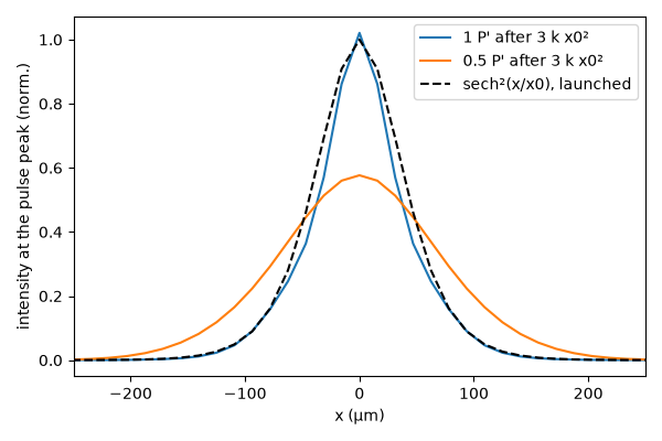
1 P': peak power 7.65e+13 W/m, energy 39.63 J/m, peak intensity ratio 1.0208
0.5 P': peak power 3.825e+13 W/m, energy 20.35 J/m, peak intensity ratio 0.5766

A line beam: diffraction and the (1+1)-D Kerr soliton#

Related reading#