Vacuum-ultraviolet dispersive-wave emission in a gas-filled capillary

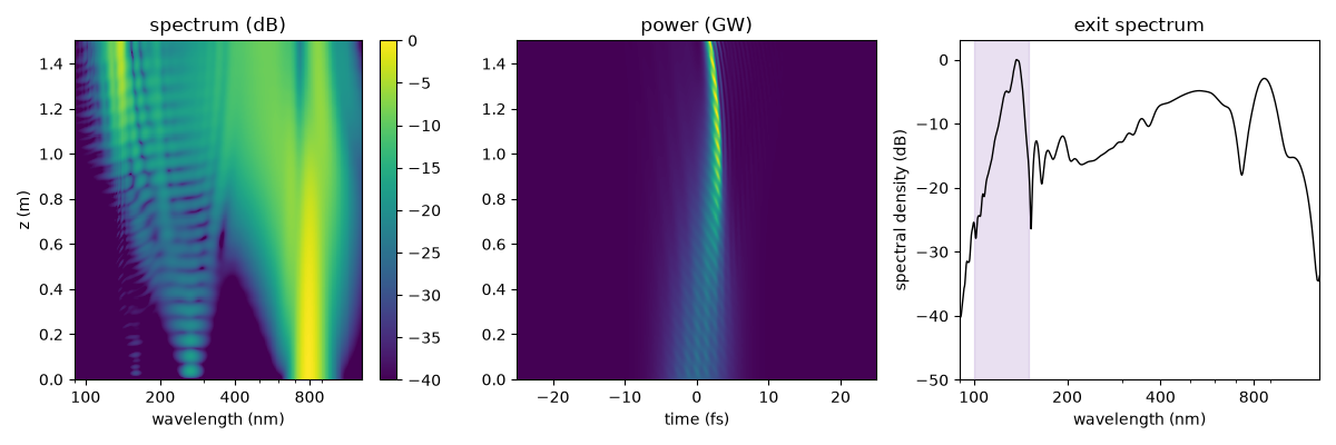
A few-cycle near-infrared pulse travelling through a hollow capillary filled with a light noble gas at low pressure can enter a higher-order soliton regime when its dispersion, duration and energy are suitable. The anomalous dispersion of the gas-filled waveguide balances self-phase modulation, the pulse compresses to a sub-cycle spike (about 1 fs), and at the point of maximum compression its spectrum extends far enough into the ultraviolet to overlap a phase-matched resonance: the soliton sheds a resonant dispersive wave (RDW) at the wavelength where the waveguide dispersion intersects the soliton’s effective propagation wavenumber, including its group-delay and nonlinear phase contributions. Because the zero-dispersion wavelength of a helium-filled capillary lies deep in the ultraviolet at sub-bar pressures, that wavelength falls in the vacuum ultraviolet, 100-150 nm here. The process is efficient, tunable with the pressure and produces pulses of a few femtoseconds; it is the basis of tabletop vacuum- and deep-ultraviolet sources.

This example runs the canonical case: a 7.5 fs, 275 uJ pulse at 800 nm in a 1.5 m long capillary of 125 um core radius, filled with helium in a pressure gradient from 0.8 bar at the entrance to vacuum at the exit. The gradient does two jobs: the pulse compresses and emits while the pressure is still high, and the dispersive wave then accumulates less material dispersion in the lower-density gas. The model does not establish the absence of absorption from every possible source. The first four HE_1m modes of the capillary are carried, so that transfer among those four channels can be followed; modes outside the retained set remain omitted; photoionisation and plasma are on.

What to look for. The spectrum broadens steadily as the pulse self-compresses. From about 0.8 m a separate band grows in the vacuum ultraviolet, between 120 and 150 nm, and it stays once the pump has passed its point of maximum compression, near 1.3 m, where the pulse is a single spike of about a femtosecond and a hundred gigawatts. At the exit a few per cent of the launched energy is in the dispersive wave.

What is approximate. The helium refractive index is optmat’s fit, qualified down to 60 nm, below the grid’s shortest wavelength (82 nm with its collar); the capillary modes are the Marcatili modes of a straight dielectric tube, whose loss in the vacuum ultraviolet is an approximation; the evacuated end is modelled by the choked steady flow, not by a true vacuum.

Begin with the paced RDW lesson. The phase-matching guide explains the wavenumber estimate, and accuracy describes the independent mode, sampling and step refinements needed for a new case.

The run

One call builds everything, runs it and returns the result. Every material is optmat’s recommended model, and the whole band lies inside the qualified ranges of the helium index and the silica wall, so the run raises no range notice.

import sys
import time
from pathlib import Path

import matplotlib.pyplot as plt
import numpy as np

from solprop.driver import prop_capillary
from solprop.processing import (
    bandpass,
    energy,
    fwhm_t,
    get_power,
    get_spectral_density,
    grid_of,
)

VUV = (100e-9, 150e-9)
"""The band the dispersive wave is counted in, m."""

started = time.perf_counter()
run = prop_capillary(
    125e-6,  # core radius, m
    1.5,  # length, m
    "He",
    (0.8, 0.0),  # bar, entrance to exit
    lambda0=800e-9,
    fwhm=7.5e-15,
    energy=275e-6,
    modes=4,
    trange=400e-15,
    wavelength_limits=(90e-9, 4e-6),
    n_save=301,
    progress="none",
)

z = np.asarray(run["z"])
window = bandpass(grid_of(run), VUV)
launched = float(np.sum(energy(run, plane=0)))
vuv = float(np.sum(energy(run, plane=-1, bandpass=window)))
print(f"launched {launched * 1e6:.0f} uJ; 100-150 nm at the exit {vuv * 1e6:.2f} uJ")
print(f"conversion efficiency {vuv / launched:.2%}")

launched 275 uJ; 100-150 nm at the exit 10.49 uJ
conversion efficiency 3.82%

Spectral and temporal evolution

The spectral energy density, summed over the modes, in decibels below its peak, and the instantaneous power in the frame moving with the pump.

wavelength, density = get_spectral_density(run, "wavelength", modes="sum")
t, power = get_power(run, modes="sum", oversampling=4)
in_band = (wavelength > 90e-9) & (wavelength < 1.3e-6)
spectrum_db = 10 * np.log10(np.maximum(density[:, in_band] / density.max(), 1e-12))

fig, (left, middle, right) = plt.subplots(1, 3, figsize=(12.0, 4.0))
image = left.pcolormesh(
    wavelength[in_band] * 1e9, z, spectrum_db, vmin=-40, vmax=0, shading="auto"
)
left.set_xscale("log")
left.set_xticks([100, 200, 400, 800], labels=["100", "200", "400", "800"])
left.set_xlabel("wavelength (nm)")
left.set_ylabel("z (m)")
left.set_title("spectrum (dB)")
fig.colorbar(image, ax=left)

near = np.abs(t) < 25e-15
middle.pcolormesh(t[near] * 1e15, z, power[:, near] * 1e-9, shading="auto")
middle.set_xlabel("time (fs)")
middle.set_title("power (GW)")

exit_db = 10 * np.log10(np.maximum(density[-1] / density[-1].max(), 1e-12))
right.plot(wavelength * 1e9, exit_db, color="k", linewidth=1.0)
right.axvspan(VUV[0] * 1e9, VUV[1] * 1e9, color="tab:purple", alpha=0.2)
right.set_xscale("log")
right.set_xlim(90, 1300)
right.set_ylim(-50, 3)
right.set_xticks([100, 200, 400, 800], labels=["100", "200", "400", "800"])
right.set_xlabel("wavelength (nm)")
right.set_ylabel("spectral density (dB)")
right.set_title("exit spectrum")
fig.tight_layout()

# The same figure illustrates the package's README. (The gallery runs the script with
# its own path in ``sys.argv[0]``.)
static = Path(sys.argv[0]).resolve().parents[2] / "_static"
if static.is_dir():
    fig.savefig(static / "readme-vuv-rdw.png", dpi=150)

The self-compressed pulse

The shortest pulse along the fibre, and where it happens.

peak = power.max(axis=1)
best = int(np.argmax(peak))
print(
    f"peak power {peak[best] * 1e-9:.0f} GW at z = {z[best]:.3f} m, "
    f"{fwhm_t(run, plane=best, modes='sum') * 1e15:.2f} fs FWHM there"
)

peak power 106 GW at z = 1.250 m, 0.98 fs FWHM there

Runtime and reproducibility

print(f"{time.perf_counter() - started:.0f} s; backend {run.metadata.backend.name}")

8 s; backend native