A frequency-dependent Kerr response

A gas’s electronic third-order response is not one number. Its hyperpolarisability depends on all four frequencies of each mixing quartet, and it rises towards the ultraviolet: argon’s Kerr coefficient at 267 nm is twice its value at 800 nm. The default carrier-kerr policy freezes it at the run’s carrier and uses that value for every process the cubic drives. Two opt-in policies of SEP 6 evaluate optmat’s whole fit instead, at the absolute frequencies of every quartet, in one broadband polarisation (A frequency-dependent electronic response):

• "gas-polynomial" evaluates the gas dispersion polynomial itself;

• "symmetric-kerr" factorises its Kerr diagonal symmetrically over the four legs, a cheaper approximation that is exact for self-phase modulation.

This tutorial compares the three on the two demonstration cases of SEP 6:

1. Deep-ultraviolet four-wave mixing in argon. A 400 nm pump and an 800 nm seed make 266.7 nm, \(\omega_s = 2\omega_p - \omega_i\), in a capillary at its linear phase-matching pressure. The declared active band lies inside argon’s electronic-response band edge, so the dispersive evaluators are supported or bounded throughout.

2. Resonant dispersive-wave emission in helium, the case of Resonant dispersive-wave propagation. Here the field reaches below helium’s two-photon resonance at a 120.3 nm fundamental, where no off-resonant model is valid. The dispersive evaluators still run it, with every leg held at the edge of helium’s data, and the band beyond the edge labelled best effort. The comparison is a sensitivity study of the vacuum-ultraviolet legs, not a qualified prediction.

What to look for. In argon, the dispersive responses make the signal grow faster at first – the generating quartet’s coefficient is 4 % above the pump’s Kerr value – but saturate earlier and lower, because the signal’s cross-phase modulation by the pump is 25 % stronger than the carrier model says, which detunes the phase matching. The two dispersive evaluators agree to about one per cent. In helium, the soliton’s own self-phase modulation is identical under all three, so the pump dynamics barely move; the dispersive wave’s energy changes by about a tenth and its centre wavelength by about a nanometre.

What is approximate. Only the electronic response differs between the runs: the linear operator, the pulse, the grid, the plasma and the backend are the same. Every run here selects backend="numba_cpu", the carrier runs too, for a like-for-like comparison: the dispersive responses run on numpy_ref, numba_cpu and the native backend’s CPU build.

Setting up

The three policies are values of MaterialSelection.electronic. Each run passes its selection with materials=, and backend="numba_cpu" explicitly: a dispersive response on a backend without it is refused, never quietly replaced.

import math
import time
import warnings

import matplotlib.pyplot as plt
import numpy as np
from scipy.optimize import brentq

from solprop.constants import C
from solprop.driver import prop_capillary
from solprop.exceptions import MaterialRangeWarning
from solprop.modes import MarcatiliMode
from solprop.physdata import MaterialSelection
from solprop.physdata.nonlinear_data import OptmatKerr
from solprop.processing import bandpass, energy, get_spectral_density, grid_of
from solprop.processing.time import moment
from solprop.pulses import GaussianPulse

started = time.perf_counter()
POLICIES = ("carrier-kerr", "symmetric-kerr", "gas-polynomial")
COLOURS = {policy: f"C{index}" for index, policy in enumerate(POLICIES)}


def wavelength_to_omega(wavelength):
    """Return the angular frequency of a vacuum wavelength."""
    return 2.0 * math.pi * C / wavelength

Argon: the phase-matching pressure

The quartet is phase matched when \(2\beta(\omega_p) = \beta(\omega_i) + \beta(\omega_s)\) in the fundamental mode. The vacuum parts cancel, so the mismatch is formed from the modes’ neff - 1, which solprop evaluates without cancellation, and its zero in pressure is found with brentq. The gas’s normal dispersion and the waveguide’s anomalous contribution balance at a few hundred millibar in a 50 um-radius capillary: this is the linear phase matching, the admitted linear model’s, which the nonlinear phases then detune.

RADIUS = 50e-6
LENGTH = 0.5
PUMP, IDLER = 400e-9, 800e-9
SIGNAL = 1.0 / (2.0 / PUMP - 1.0 / IDLER)
omega = wavelength_to_omega(np.array([PUMP, IDLER, SIGNAL]))


def mismatch(pressure):
    """Return 2 beta_p - beta_i - beta_s of the HE_11 mode, 1/m."""
    mode = MarcatiliMode(RADIUS, "Ar", pressure)
    excess = omega / C * mode.neff_minus_one(omega).real
    return float(2.0 * excess[0] - excess[1] - excess[2])


with warnings.catch_warnings():
    warnings.simplefilter("ignore", MaterialRangeWarning)
    PRESSURE = brentq(mismatch, 0.01, 5.0, xtol=1e-9)
print(f"signal {SIGNAL * 1e9:.1f} nm; phase matched at {PRESSURE * 1e3:.1f} mbar")

signal 266.7 nm; phase matched at 209.4 mbar

Argon: the coefficients of the quartets that matter

Before any propagation, the per-particle coefficient each policy assigns to the quartets this case drives, from optmat’s fit of argon in SI (DispersiveKerrModel). A quartet is four signed frequencies, the output counted negative; only their squares enter the polynomial \(\gamma_0[1 + aS_2 + bS_2^2 + b'S_4]\), and the symmetric model is the product \(\gamma_0\prod_j g(\nu_j)\) with \(g = [\gamma_K(\nu)/\gamma_0]^{1/4}\). Every leg is first held at argon’s leg bound, 215.9 nm, which no frequency here reaches. The output-only column multiplies by the output’s Kerr value, the construction SEP 6 rejects, for contrast.

argon = OptmatKerr("Ar").dispersive_model()


def kerr_value(wavelength):
    """Return argon's bounded Kerr diagonal at a wavelength, per its static value."""
    return float(argon.kerr_ratio(argon.leg_weight(wavelength_to_omega(wavelength))))


def coefficients(output, legs):
    """Return the polynomial, symmetric and output-only coefficients of a quartet."""
    wavelengths = np.array([output, *legs])
    polynomial = float(argon.gamma3(1.0 / wavelengths)) / argon.gamma3_static
    symmetric = math.prod(kerr_value(one) ** 0.25 for one in wavelengths)
    return polynomial, symmetric, kerr_value(output)


QUARTETS = {
    "400 + 400 - 800 -> 266.7 (the signal)": (SIGNAL, (PUMP, PUMP, IDLER)),
    "SPM of 400 (the pump)": (PUMP, (PUMP, PUMP, PUMP)),
    "XPM of 266.7 by 400": (SIGNAL, (SIGNAL, PUMP, PUMP)),
    "SPM of 266.7": (SIGNAL, (SIGNAL, SIGNAL, SIGNAL)),
}
carrier = kerr_value(PUMP)
HEADER = ("poly/K(800)", "carrier", "sym.", "out")
print(
    f"{'quartet (nm)':40s} {HEADER[0]:>11s} " + " ".join(f"{x:>7s}" for x in HEADER[1:])
)
for name, (output, legs) in QUARTETS.items():
    polynomial, symmetric, output_only = coefficients(output, legs)
    errors = (carrier, symmetric, output_only)
    print(
        f"{name:40s} {polynomial / kerr_value(IDLER):11.3f} "
        + " ".join(f"{100 * (value / polynomial - 1):+7.2f}" for value in errors)
    )
print("errors in per cent of the polynomial; the carrier is the pump's Kerr value")

quartet (nm)                             poly/K(800) carrier    sym.     out
400 + 400 - 800 -> 266.7 (the signal)          1.345   -4.25   +0.56  +50.00
SPM of 400 (the pump)                          1.288   +0.00   +0.00   +0.00
XPM of 266.7 by 400                            1.612  -20.13   -0.03  +25.13
SPM of 266.7                                   2.018  -36.17   +0.00   -0.00
errors in per cent of the polynomial; the carrier is the pump's Kerr value

The carrier model is 4 % low for the generating quartet – a small error – but 20 % low for the cross-phase modulation of the signal by the pump, and 36 % low for the signal’s own self-phase modulation. The symmetric model is within 0.6 % of the polynomial on all of them, and exact on the Kerr diagonal. The output-only construction is wrong by up to 50 %.

Argon: three propagations

Half a metre of capillary, 10 uJ in each of a 30 fs pump and seed. The grid’s shortest wavelength, 210 nm, keeps its active band (to 191 nm) inside argon’s band edge at 189.4 nm, so the run has no best-effort region.

def fwm_run(policy):
    """Propagate the argon DUV case under one electronic policy."""
    with warnings.catch_warnings():
        # The padded grid reaches beyond the qualified range of the gas index; each run
        # says so once, which is not this tutorial's point.
        warnings.simplefilter("ignore", MaterialRangeWarning)
        return prop_capillary(
            RADIUS,
            LENGTH,
            "Ar",
            PRESSURE,
            lambda0=PUMP,
            pulses=[
                GaussianPulse(wavelength=PUMP, fwhm=30e-15, energy=10e-6),
                GaussianPulse(wavelength=IDLER, fwhm=30e-15, energy=10e-6),
            ],
            wavelength_limits=(210e-9, 2e-6),
            trange=250e-15,
            n_save=26,
            backend="numba_cpu",
            materials=MaterialSelection(electronic=policy),
            progress="none",
        )


fwm = {policy: fwm_run(policy) for policy in POLICIES}

What each run recorded. The manifest of a dispersive run names its law and, for each gas, the regions of its active band: argon’s is supported down to the leg bound and bounded beyond it, and nothing is best effort.

(entry,) = fwm["gas-polynomial"].metadata.materials.electronic
regions = entry["regions"]
for name in ("supported", "bounded", "best_effort"):
    span = regions[name]
    text = "none" if span is None else f"{span[0] * 1e9:.1f}-{span[1] * 1e9:.0f} nm"
    print(f"{name:12s} {text}")

supported    215.9-4000 nm
bounded      190.9-216 nm
best_effort  none

The signal’s energy along the fibre and its spectrum at the exit. The band is 250-285 nm, which holds the signal and nothing else.

z = np.asarray(fwm["carrier-kerr"]["z"])
band = bandpass(grid_of(fwm["carrier-kerr"]), (250e-9, 285e-9))


def band_energies(run, window):
    """Return a band's energy at every saved plane, J."""
    planes = np.asarray(run["z"]).size
    return np.array(
        [
            float(np.sum(energy(run, plane=index, bandpass=window)))
            for index in range(planes)
        ]
    )


fig, (left, right) = plt.subplots(1, 2, figsize=(10.0, 3.6), layout="constrained")
signal = {policy: band_energies(run, band) for policy, run in fwm.items()}
for policy, run in fwm.items():
    left.plot(z, 1e6 * signal[policy], lw=1.6, color=COLOURS[policy], label=policy)
    wavelength, density = get_spectral_density(
        run, "wavelength", plane=-1, modes="sum", spec_range=(245e-9, 290e-9)
    )
    right.plot(
        1e9 * wavelength, 1e-3 * density, lw=1.4, color=COLOURS[policy], label=policy
    )
left.set_xlabel("z (m)")
left.set_ylabel("250-285 nm energy (uJ)")
left.legend(frameon=False)
right.set_xlabel("wavelength (nm)")
right.set_ylabel("spectral energy density at the exit (nJ/nm)")
right.legend(frameon=False)

for policy in POLICIES:
    peak = int(np.argmax(signal[policy]))
    print(
        f"{policy:15s} largest {1e6 * signal[policy][peak]:.2f} uJ at "
        f"{z[peak]:.2f} m; at the exit {1e6 * signal[policy][-1]:.2f} uJ"
    )

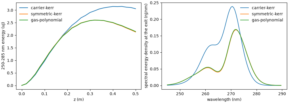
carrier-kerr    largest 3.15 uJ at 0.44 m; at the exit 3.06 uJ
symmetric-kerr  largest 2.60 uJ at 0.32 m; at the exit 2.13 uJ
gas-polynomial  largest 2.60 uJ at 0.32 m; at the exit 2.15 uJ

In the first few centimetres, where the pump is undepleted and the phase matching is still the linear one, the signal’s energy goes as the square of the generating quartet’s coefficient: the dispersive runs are 7-8 % ahead, twice the 4 % above. Beyond that, the stronger cross-phase modulation of the signal by the pump moves it off phase matching sooner. At the exit the carrier model overestimates the signal by about 40 %: the error that matters here is not the generating coefficient but the nonlinear phases. The symmetric and polynomial evaluators stay within about one per cent of each other along the whole fibre.

Helium: the dispersive wave

The case of Resonant dispersive-wave propagation, unchanged but for the backend and policy: one metre of 125 um-radius capillary, helium falling from 1.2 bar to vacuum, 275 uJ in 7.5 fs at 800 nm, two modes.

VUV = (100e-9, 140e-9)


def rdw_run(policy):
    """Propagate the helium RDW case under one electronic policy."""
    with warnings.catch_warnings():
        warnings.simplefilter("ignore", MaterialRangeWarning)
        return prop_capillary(
            125e-6,
            1.0,
            "He",
            (1.2, 0.0),
            lambda0=800e-9,
            wavelength_limits=(100e-9, 1.5e-6),
            trange=200e-15,
            fwhm=7.5e-15,
            energy=275e-6,
            modes=2,
            n_save=51,
            backend="numba_cpu",
            materials=MaterialSelection(electronic=policy),
            progress="none",
        )


rdw = {policy: rdw_run(policy) for policy in POLICIES}

Helium’s regions: its data reach legs down to 151.9 nm, its band edge – the two-photon resonance – is at 120.3 nm, and the grid’s active band reaches 90.9 nm. So the dispersive wave’s band, 100-140 nm, is part bounded and part best effort.

(entry,) = rdw["gas-polynomial"].metadata.materials.electronic
helium_regions = entry["regions"]
for name in ("supported", "bounded", "best_effort"):
    span = helium_regions[name]
    print(f"{name:12s} {span[0] * 1e9:.1f}-{span[1] * 1e9:.1f} nm")

supported    151.9-3000.0 nm
bounded      120.3-151.9 nm
best_effort  90.9-120.3 nm

The dispersive wave’s energy along the fibre, and the exit spectrum with the bounded (light) and best-effort (dark) bands shaded. The centre wavelength is the energy-weighted mean frequency of the 100-140 nm band, expressed as a wavelength.

z_rdw = np.asarray(rdw["carrier-kerr"]["z"])
window = bandpass(grid_of(rdw["carrier-kerr"]), VUV)


def centre_wavelength(run):
    """Return the energy-weighted centre of the VUV band at the exit, m."""
    band_omega = (wavelength_to_omega(VUV[1]), wavelength_to_omega(VUV[0]))
    frequency, density = get_spectral_density(
        run, "omega", plane=-1, modes="sum", spec_range=band_omega
    )
    return wavelength_to_omega(moment(frequency, density))


fig, (left, right) = plt.subplots(1, 2, figsize=(10.0, 3.6), layout="constrained")
for name, shade in (("bounded", "0.9"), ("best_effort", "0.75")):
    low, high = helium_regions[name]
    right.axvspan(
        1e9 * low, 1e9 * high, color=shade, lw=0, label=name.replace("_", " ")
    )
results = {}
for policy, run in rdw.items():
    vuv = band_energies(run, window)
    results[policy] = (vuv[-1], centre_wavelength(run))
    left.plot(z_rdw, 1e6 * vuv, lw=1.6, color=COLOURS[policy], label=policy)
    wavelength, density = get_spectral_density(
        run, "wavelength", plane=-1, modes="sum", spec_range=(90e-9, 400e-9)
    )
    right.semilogy(
        1e9 * wavelength,
        density / density.max(),
        lw=1.0,
        color=COLOURS[policy],
        label=policy,
    )
left.set_xlabel("z (m)")
left.set_ylabel("100-140 nm energy (uJ)")
left.legend(frameon=False)
right.set_ylim(1e-4, 2.0)
right.set_xlabel("wavelength (nm)")
right.set_ylabel("exit spectrum (normalised)")
right.legend(frameon=False, fontsize="small", ncols=2)

reference = results["gas-polynomial"]
for policy, (band_energy, centre) in results.items():
    print(
        f"{policy:15s} 100-140 nm {1e6 * band_energy:.2f} uJ "
        f"({100 * (band_energy / reference[0] - 1):+.1f} %), "
        f"centre {1e9 * centre:.2f} nm"
    )

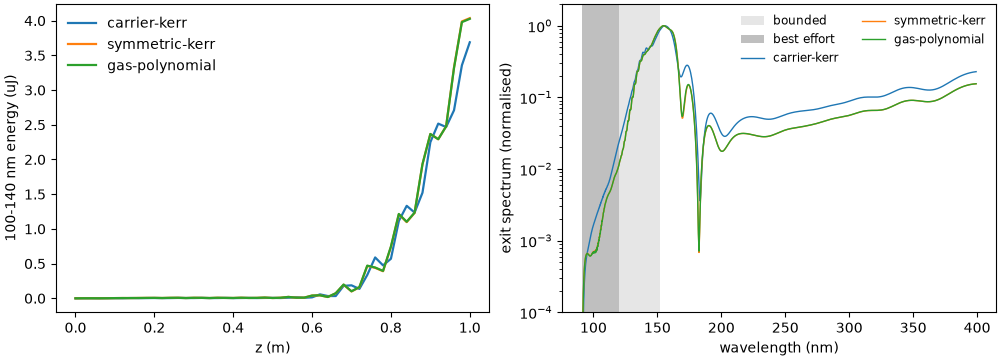
carrier-kerr    100-140 nm 3.69 uJ (-8.4 %), centre 133.16 nm
symmetric-kerr  100-140 nm 4.04 uJ (+0.2 %), centre 134.16 nm
gas-polynomial  100-140 nm 4.03 uJ (+0.0 %), centre 134.16 nm

The soliton’s self-phase modulation at 800 nm keeps its carrier value under every policy, and the quartets of its broadened wings lie inside helium’s data, so the pump compresses in much the same place. The dispersive wave’s wavelength is set by phase matching to that soliton and moves by about a nanometre. Its energy moves by about a tenth: the quartets that generate it carry a vacuum-ultraviolet leg, held at the value of helium’s leg bound (151.9 nm) by the dispersive evaluators and at the 800 nm value by the carrier model. Between 120.3 and 151.9 nm the bounded value is a held-coefficient approximation, not a lower bound on the emitted energy; below 120.3 nm neither off-resonant treatment is qualified. The spread between them is the sensitivity of this observable to that unknown, and a resonant helium response – such as the TDSE coupling of TDSE response in a helium capillary – requires its own atomic, temporal and spatial qualification; it is not automatically an accurate reference for this propagation problem.

Runtime and reproducibility

print(f"{time.perf_counter() - started:.0f} s on numba_cpu")

39 s on numba_cpu

Related reading

Continue with A frequency-dependent electronic response for the model, options and limits, and Assessing numerical accuracy for convergence checks. For a paced propagation lesson, return to Resonant dispersive-wave propagation.