Photoionisation-induced soliton blue-shift

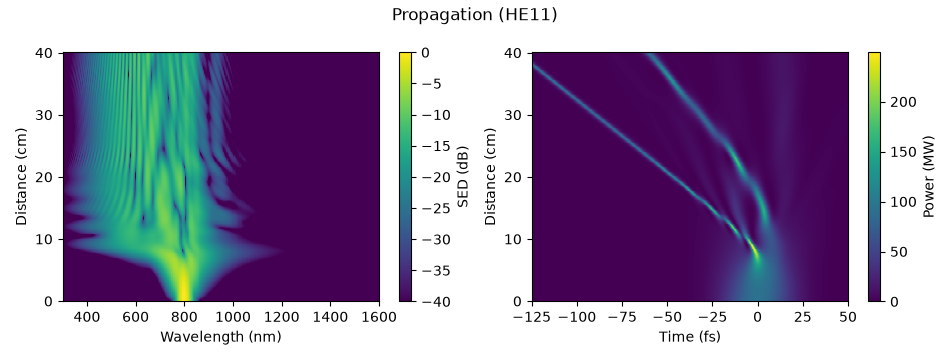
When a soliton self-compresses to intensities of order \(10^{14}\,\text{W/cm}^2\) it can ionise the gas; the fraction depends on species, pulse duration and the selected rate model. The free electrons it creates lower the refractive index, and because they accumulate during the pulse the index falls along it: the trailing part of the pulse sees a lower index than the leading part, and the resulting phase shifts its frequency upwards. A soliton that is ionising therefore shifts its own spectrum to the blue – the opposite of the Raman self-frequency shift – and accelerates, so that its trajectory in time bends towards earlier arrival. The shift is self-limiting: the blue-shifted soliton sees a different dispersion and its intensity, and hence the ionisation, falls. The effect was a signature of the first experiments on plasma-soliton dynamics in gas-filled hollow-core photonic crystal fibres, and it is readily reproduced in small-core capillaries.

Here a 30 fs, 3 uJ pulse at 800 nm travels 0.4 m through a 13 um-radius capillary filled with argon at 1.7 bar, with its loss switched off (standing in for a low-loss hollow-core fibre). Ionisation uses optmat’s recommended rate for argon (a Perelomov–Popov–Terent’ev rate), chosen automatically.

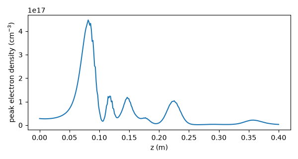
What to look for. The pulse self-compresses over the first eight centimetres or so and ionises the gas; over the next few centimetres its spectrum moves bodily to shorter wavelengths – the centroid from 800 nm to about 640 nm – while the pulse bends towards earlier times, and then the shift stops as the intensity falls. The peak electron density along the fibre shows where it happened.

What is approximate. The capillary dispersion stands in for a hollow-core fibre; only the fundamental mode is carried.

This is panel (f) of the survey of nonlinear processes in the review by Travers et al.

For the rate and its uncertainty see Strong-field ionisation; for population and current accounting see Carrier-resolved plasma response. The filament lesson shows plasma acting together with transverse self-focusing.

The run

import time

import matplotlib.pyplot as plt
import numpy as np

from solprop.constants import C
from solprop.driver import prop_capillary
from solprop.plotting import prop_2d, spec_1d, time_1d
from solprop.processing import get_spectral_density

started = time.perf_counter()
run = prop_capillary(
    13e-6,
    0.4,
    "Ar",
    1.7,
    lambda0=800e-9,
    fwhm=30e-15,
    energy=3e-6,
    loss=False,
    trange=400e-15,
    wavelength_limits=(300e-9, 4e-6),
    n_save=301,
    progress="none",
)

Spectral and temporal evolution

figures = prop_2d(
    run,
    "wavelength",
    wavelength_range=(300e-9, 1.6e-6),
    trange=(-125e-15, 50e-15),
    db_min=-40,
)
figures[-1].set_size_inches(9.5, 3.6)
figures[-1].tight_layout()

The output, and the plasma

fig, (left, right) = plt.subplots(1, 2, figsize=(10.0, 3.6))
time_1d(run, z=[0.0, 0.4], trange=(-125e-15, 50e-15), ax=left)
spec_1d(run, z=[0.0, 0.4], ax=right, wavelength_range=(300e-9, 1.6e-6))
fig.tight_layout()

z = np.asarray(run["z"])
omega, spectral = get_spectral_density(run, "omega")
centroid = 2 * np.pi * C * np.sum(spectral, axis=1) / np.sum(spectral * omega, axis=1)
print(f"spectral centroid {centroid[0] * 1e9:.0f} nm -> {centroid[-1] * 1e9:.0f} nm")
density = np.asarray(run["stats/electron_density"]).reshape(z.size, -1).max(axis=1)
fig, ax = plt.subplots(figsize=(6.0, 3.2))
ax.plot(z, density * 1e-6)
ax.set_xlabel("z (m)")
ax.set_ylabel("peak electron density (cm$^{-3}$)")
fig.tight_layout()
print(
    f"peak electron density {density.max() * 1e-6:.2e} cm^-3 at z = "
    f"{z[int(np.argmax(density))]:.3f} m"
)

• 
• 

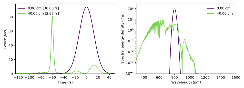
spectral centroid 800 nm -> 637 nm
peak electron density 4.48e+17 cm^-3 at z = 0.081 m

Runtime and reproducibility

print(f"{time.perf_counter() - started:.0f} s; backend {run.metadata.backend.name}")

12 s; backend native